R Fundamentals Part 1

Welcome to Data Science with R!

Oliver Bonham-Carter

Welcome to CS301!

What You’ll Learn Today

• Course Overview — What makes this course exciting
• R & RStudio Setup — Getting started
• Variables & Data Types — Storing information
• Vectors — R’s fundamental data structure
• Basic Operations — Math & logic in R
• Interactive Tools — Hands-on code generators!

Get ready for an amazing journey into data science! 🌟

Careers in Data Science

• Data Analyst: Works with data to find trends and create reports. They use tools like Excel, SQL, and visualization software.

• Data Scientist: Builds models to predict outcomes. They use programming languages like Python or R and machine learning techniques.

• Data Engineer: Designs and builds systems to collect and store data. They work with databases and big data tools.

• Machine Learning Engineer: Creates algorithms that learn from data. They focus on deploying models in real-world applications.

• Business Intelligence Analyst: Translates data into business insights. They create dashboards and help decision-makers.

Skills for Careers in DS?

• Programming: Learn Python or R. These languages help you clean and analyze data.

• Statistics: Understand basic statistics to interpret data correctly.

• Data Visualization: Use tools like Tableau or Power BI to create clear charts.

• Machine Learning: Know how to build and test predictive models.

• Communication: Explain your findings clearly to non-technical people.

• Problem Solving: Think critically to find the best solutions.

Note

Plan your work, work your plan!

Salaries in Data Science

Important

• Salary by Experience
  • Level Entry-Level (0–2 years): $80,000 – $98,000
  • Mid-Level (3–5 years): $110,000 – $150,000
  • Senior / Lead (5+ years): $160,000 – $220,000+ (including equity and bonuses)
• Top-Paying Cities
  • San Francisco, CA: ~$171,870 per year
  • Seattle, WA: ~$156,328 per year
  • New York, NY: ~$137,426 per year

Salary info: USNews

Tentative Course Roadmap

R Foundations

• Programming basics
• Data manipulation
• Visualization
• Functions & control flow
• Fun with R!

Advanced Topics

• SQL & databases
• Big data with R
• Shiny applications
• Python integration
• Probability & distributions

ML and Beyond

• Hypothesis testing
• Regression models
• Decision trees
• Neural networks
• Final projects

Today we start with the fundamentals — the building blocks of everything else!

Part 1: Getting Started with R

Why Data Science with R?

Important

R: Purpose-Built for Data

R was designed specifically for statistical computing and data analysis:

• Statistical Power — Thousands of built-in functions
• Visualization Excellence — Beautiful plots with ggplot2
• Data Wrangling — Powerful tidyverse ecosystem
• Industry Standard — Used at Google, Facebook, Twitter, academia
• Career Ready — High demand for R skills in data science

The Big Picture: You will learn R for data analysis, but we will also introduce some Python later to show you how they complement each other.

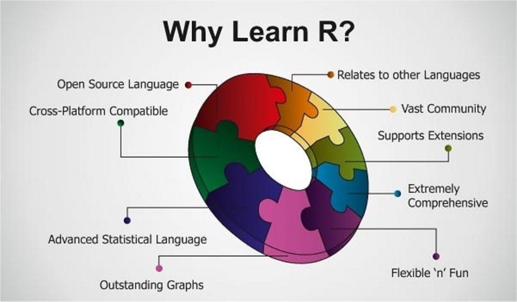
So, Why Learn this Language?

While you are waiting for the install to complete, here’s more fun facts about R and why it is a great language to learn for data science!

R : The Programming Language (the engine)

R is a programming language for statistical computing and data analysis.

• R was named after its creators: Ross Ihaka and Robert Gentleman, whose names both start with “R.”
• R is especially popular for statistics and data visualization.
• It has thousands of packages that make it useful for everything from analyzing data to creating colorful graphs.
• R can make some seriously impressive graphics. Packages like ggplot2 allow users to create professional-looking charts with just a few lines of code.

RStudio : The IDE (the dashboard)

RStudio is an integrated development environment (IDE) for R. It provides a user-friendly interface for writing and executing R code.

• RStudio is an IDE (Integrated Development Environment) designed to make working with R easier. It puts your code, graphs, files, and data tools all in one place.
• RStudio was created by a company originally called RStudio. The company later changed its name to Posit as it expanded its support for other data-science tools.
• RStudio makes packages easier to use. You can install and manage R packages, run code, and view documentation without having to do everything from the command line.
• There is a cloud version called Posit Cloud. It lets you use R and other data-science tools through a web browser without installing everything on your computer.

Installing R & RStudio

Download R

1. Visit CRAN Download Site

2. Click “Download R”

3. Choose your CRAN mirror (if asked, choose one close to your geographical location)

4. Select your OS, download the installer, and follow the installation instructions

Latest version: R 4.5.x: See R Project

Download RStudio

1. Visit posit.co
2. Download RStudio Desktop (Open Source and Free)
3. Install RStudio after R has been installed

• Note: RStudio is not the programming language. Instead, it is similar to an IDE that manages R programming. <!– RStudio gives you:

• Script editor

• Console

• Plots & visualizations

• Environment viewer –>

Your RStudio Environment

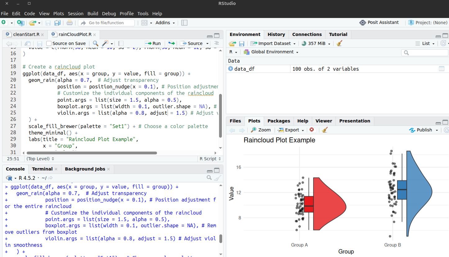
Your RStudio Environment

The Four Panes

Top-Left: Script Editor — Write & save your code
Bottom-Left: Console — Execute commands interactively
Top-Right: Environment — See your variables & data
Bottom-Right: Files, Plots, Help, Packages

Try It Out! Open RStudio and type in the console:

# Your first R command!
print("Hello, Data Science!")

# Basic math
2 + 2
10 * 5
sqrt(16)

Pro Tip: The console shows > when ready for input. If you see +, R is waiting for you to complete a command!

Part 2: Variables & Data Types

Creating Variables

Important

Variables Store Information

In R, we use <- (or =) to assign values to variables

# Creating variables
name <- "Alice"
age <- 25
height_cm <- 170.5
is_student <- TRUE

# Using variables
age + 5              # Result: 30
height_cm / 100      # Convert to meters: 1.705

# You can update variables
age <- age + 1       # Alice had a birthday!
age                  # Now 26

Tip

Style Guide: Use <- for assignment (not =). Use descriptive names with underscores: student_count, not sc or studentCount.

Interactive: Variable Creator

🔧 Variable Creator & Tester

Variable Name:

Data Type: Numeric Character (Text) Logical (TRUE/FALSE)

Value:

Click "Create Variable" to generate R code!

R Data Types: The Big Four

Numeric

# Numbers (integers & decimals)
age <- 25
price <- 19.99
temperature <- -5.2

# Check type
class(age)       # "numeric"
typeof(price)    # "double"
is.numeric(age)  # TRUE

Character

# Text strings (use quotes)
name <- "Alice"
city <- 'Boston'
message <- "Hello, R!"

# Check type
class(name)        # "character"
nchar(name)        # 5 characters
toupper(name)      # "ALICE"

Logical

# TRUE or FALSE (Boolean)
is_student <- TRUE
passed_exam <- FALSE
eligible <- TRUE

# Check type
class(is_student)  # "logical"
!is_student        # NOT: FALSE
TRUE & FALSE       # AND: FALSE
TRUE | FALSE       # OR: TRUE

Special Values

# Missing data
missing <- NA      # Not Available

# Infinity
infinity <- Inf
neg_inf <- -Inf

# Not a Number
undefined <- NaN   # 0/0

# NULL (empty)
empty <- NULL

Part 3: Vectors - R’s Superpower

What are Vectors?

Vectors: Collections of Values

A vector is a sequence of elements of the same type. This is R’s most fundamental data structure!

# Creating vectors with c() (combine function)
ages <- c(25, 30, 22, 35, 28)
names <- c("Alice", "Bob", "Carol", "David", "Eve")
passed <- c(TRUE, TRUE, FALSE, TRUE, TRUE)

# Vectors can only hold ONE type
mixed <- c(1, 2, "three", 4)  # Everything becomes character!
class(mixed)  # "character"

# Sequences
nums1 <- 1:10                    # 1 2 3 4 5 6 7 8 9 10
nums2 <- seq(0, 1, by = 0.1)    # 0.0 0.1 0.2 ... 1.0
nums3 <- seq(1, 10, length = 5) # 1.00 3.25 5.50 7.75 10.00

# Repetition
zeros <- rep(0, 5)               # 0 0 0 0 0
pattern <- rep(c(1, 2), 3)       # 1 2 1 2 1 2

Vector Operations: The Magic

Vectorization: R’s Secret Weapon

Operations apply to ALL elements at once — no loops needed!

# Create a vector
prices <- c(10, 20, 30, 40, 50)

# Vectorized operations (work on ALL elements!)
prices * 2           # 20 40 60 80 100
prices + 5           # 15 25 35 45 55
prices / 10          # 1 2 3 4 5
sqrt(prices)         # 3.16 4.47 5.48 6.32 7.07

# Element-wise operations
prices1 <- c(10, 20, 30)
prices2 <- c(5, 10, 15)
prices1 + prices2    # 15 30 45
prices1 * prices2    # 50 200 450

# Statistical functions
mean(prices)         # 30
median(prices)       # 30
sum(prices)          # 150
sd(prices)           # Standard deviation: 15.81

Interactive: Vector Operation Builder

🎯 Vector Builder & Calculator

Vector 1 (comma-separated):

Operation: Statistics (mean, sum, etc.) Transform (square, sqrt, log) Add Scalar Multiply Scalar Combine with Vector 2

Scalar Value:

Vector 2 (comma-separated):

Enter vector values and select an operation!

Accessing Vector Elements

Indexing: Getting Specific Elements

R uses 1-based indexing (unlike Python’s 0-based)

Positive Indexing

fruits <- c("apple", "banana", 
            "cherry", "date")

# Single element
fruits[1]          # "apple"
fruits[3]          # "cherry"

# Multiple elements
fruits[c(1, 3)]    # "apple" "cherry"
fruits[2:4]        # "banana" to "date"

# By logical vector
fruits[c(T, F, T, F)]
# "apple" "cherry"

Negative Indexing

# Exclude elements
fruits[-1]         # All except first
fruits[-c(1, 3)]   # Exclude 1st & 3rd

# Logical conditions
scores <- c(85, 92, 78, 95, 88)

scores > 90        # T T F T F
scores[scores > 90] # 92 95

high_scores <- scores[scores >= 85]
# 85 92 95 88

Part 4: Basic Operations

Arithmetic Operations

Basic Math

# Standard operations
10 + 5         # Addition: 15
10 - 5         # Subtraction: 5
10 * 5         # Multiplication: 50
10 / 5         # Division: 2
10 ^ 2         # Power: 100
10 %% 3        # Modulo: 1
10 %/% 3       # Integer division: 3

# Order of operations
2 + 3 * 4      # 14 (not 20!)
(2 + 3) * 4    # 20

Mathematical Functions

# Common functions
sqrt(16)           # 4
abs(-5)            # 5
round(3.14159, 2)  # 3.14
ceiling(3.2)       # 4
floor(3.9)         # 3
log(10)            # 2.302585
log10(100)         # 2
exp(1)             # 2.718282

# Trigonometry
sin(pi/2)          # 1
cos(0)             # 1

Comparison & Logical Operations

Comparisons

# Comparison operators
5 == 5         # Equal: TRUE
5 != 3         # Not equal: TRUE
5 > 3          # Greater: TRUE
5 < 3          # Less: FALSE
5 >= 5         # Greater/equal: TRUE
5 <= 4         # Less/equal: FALSE

# With vectors (element-wise!)
x <- c(1, 5, 9)
x > 4          # FALSE TRUE TRUE
x == 5         # FALSE TRUE FALSE

Logical Operators

# AND, OR, NOT
TRUE & TRUE    # TRUE
TRUE & FALSE   # FALSE
TRUE | FALSE   # TRUE
!TRUE          # FALSE

# With variables
age <- 25
age >= 18 & age < 65   # TRUE

score <- 85
score >= 90 | score < 60  # FALSE

# Element-wise with vectors
x <- c(1, 5, 9)
x > 3 & x < 8  # FALSE TRUE FALSE

Interactive: Expression Evaluator

🧮 R Expression Evaluator

Expression Type: Arithmetic Comparison Logical Vector Operations

Try These Examples: -- Select Example --

Enter Your R Expression:

Enter an expression and click "Evaluate"!

Recap & Up Next

What We Learned Today

R & RStudio setup Variables and data types (numeric, character, logical) Vectors: creation, operations, indexing Arithmetic, comparison, and logical operations Interactive tools for hands-on learning

Up Next

Practice: Create vectors, try operations, experiment!
Install: Make sure R and RStudio are working
Preview: We’ll explore data structures (lists, data frames, matrices)

Quick Challenges!

Challenge 1: Output Prediction

What will this code return?

x <- c(10, 20, 30, 40, 50)
mean(x[x > 25])

25

30

40

35

Challenge 2: Variable Types

What will be the type of variable x after running: x <- c(1, 2, "3")?

numeric

character

mixed

logical

Challenge 3: Vector Operations

If x <- c(10, 20, 30) and y <- c(1, 2), what does x + y produce?

Error: vectors different lengths

11, 22, 31 (with warning)

11, 22, 30

31 (sum of all elements)

Challenge 4: Logical Indexing

Given scores <- c(85, 92, 78, 95, 88), which code gets scores above 90?

scores[>90]

scores[scores > 90]

scores$>90

filter(scores > 90)

Challenge 5: Code Writing

Write code to create a vector of even numbers from 2 to 20, then find their mean.

Solution:
# Method 1: Using seq()
evens <- seq(2, 20, by = 2)
mean(evens)

# Method 2: Using sequence and filtering
evens <- (1:10) * 2
mean(evens)

# Result: 11

Bonus: Quick Reference Card

Variable Assignment

x <- 10        # Assign
x = 10         # Also works
10 -> x        # Rarely used

Vector Creation

c(1,2,3)       # Combine
1:10           # Sequence
seq(1,10,2)    # Custom seq
rep(5, 3)      # Repeat

Vector Access

x[1]           # First element
x[c(1,3)]      # Multiple
x[2:4]         # Range
x[-1]          # Exclude
x[x>5]         # Logical

Arithmetic

+ - * /        # Basic
^ or **        # Power
%% %/%         # Modulo, int div
sqrt() abs()   # Functions
log() exp()    # Logarithms

Comparisons

== !=          # Equal, not equal
< > <= >=      # Comparisons

Logical

& |            # AND, OR
!              # NOT
&&  ||         # Short-circuit

Stats

mean() median()
sum() prod()
min() max()
sd() var()