R Fundamentals Part 2

Data Structures & Advanced Concepts

CS301 - Data Science with R

What’s on for today?

Today’s Journey

📋 Lists — Flexible containers for mixed data
📊 Matrices — Two-dimensional numeric data
🗂️ Data Frames — The heart of data science in R
📁 Reading Data — Getting data into R (CSV files)
🎮 Interactive Tools — Build data frames & matrices visually!

Last week: Variables & Vectors | This week: Complex data structures! 🏗️

Quick Recap: Vectors

# Remember vectors? All elements same type
numbers <- c(1, 2, 3, 4, 5)
names <- c("Alice", "Bob", "Carol")
flags <- c(TRUE, FALSE, TRUE)

# Vectorized operations
numbers * 2         # 2 4 6 8 10
mean(numbers)       # 3
numbers[numbers > 3] # 4 5

Important

Today’s Challenge: What if we need to store different types together? Or organize data in 2D? That’s where lists, matrices, and data frames come in! 🚀

Part 1: Lists - The Flexible Container

What Are Lists?

Lists: R’s Swiss Army Knife 🔧

Lists can hold different types of data, even other lists!

Creating Lists

# Simple list
person <- list(
  name = "Alice",
  age = 25,
  scores = c(90, 85, 92),
  passed = TRUE
)

# Access by name
person$name      # "Alice"
person$age       # 25
person$scores    # 90 85 92

# Access by index
person[[1]]      # "Alice"
person[[3]]      # 90 85 92

Why Lists?

# Vectors force one type
mixed_vec <- c(1, "two", TRUE)
mixed_vec
# "1" "two" "TRUE" - all character!

# Lists preserve types
mixed_list <- list(1, "two", TRUE)
mixed_list[[1]]  # numeric: 1
mixed_list[[2]]  # character: "two"
mixed_list[[3]]  # logical: TRUE

# Lists can be nested!
nested <- list(
  data = list(x = 1:5, y = 6:10),
  meta = list(source = "experiment")
)

Interactive: List Builder

🔧 Interactive List Creator

Add elements and click "Generate Code"!

Part 2: Matrices - 2D Numeric Data

Creating Matrices

Matrices: Rows × Columns of Numbers

Matrices are 2-dimensional arrays of the same type (usually numeric)

By Values

# Create matrix from vector
m <- matrix(
  1:12,           # Data
  nrow = 3,       # 3 rows
  ncol = 4        # 4 columns
)

m
#      [,1] [,2] [,3] [,4]
# [1,]    1    4    7   10
# [2,]    2    5    8   11
# [3,]    3    6    9   12

# Fill by row instead
matrix(1:12, nrow=3, byrow=TRUE)
#      [,1] [,2] [,3] [,4]
# [1,]    1    2    3    4
# [2,]    5    6    7    8
# [3,]    9   10   11   12

By Binding Vectors

# Column binding
c1 <- c(1, 2, 3)
c2 <- c(4, 5, 6)
cbind(c1, c2)
#      c1 c2
# [1,]  1  4
# [2,]  2  5
# [3,]  3  6

# Row binding
r1 <- c(1, 2, 3)
r2 <- c(4, 5, 6)
rbind(r1, r2)
#    [,1] [,2] [,3]
# r1    1    2    3
# r2    4    5    6

Matrix Operations

# Create sample matrices
A <- matrix(1:6, nrow=2, ncol=3)
B <- matrix(7:12, nrow=2, ncol=3)

# Element-wise operations
A + B                # Add corresponding elements
A * B                # Multiply corresponding elements
A / B                # Divide corresponding elements

# Matrix multiplication (dimensions must match!)
C <- matrix(1:6, nrow=3, ncol=2)
A %*% C              # True matrix multiplication

# Transpose
t(A)                 # Flip rows and columns

# Other operations
nrow(A)              # Number of rows: 2
ncol(A)              # Number of columns: 3
dim(A)               # Dimensions: 2 3

Accessing Matrix Elements

# Create matrix
m <- matrix(1:12, nrow=3, ncol=4)

# Single element
m[1, 2]              # Row 1, Column 2: 4
m[3, 4]              # Row 3, Column 4: 12

# Entire row or column
m[1, ]               # First row: 1 4 7 10
m[, 2]               # Second column: 4 5 6

# Multiple rows/columns
m[1:2, ]             # Rows 1-2
m[, c(1, 3)]         # Columns 1 and 3

# Submatrix
m[1:2, 2:3]          # Top-left 2×2 of middle columns

# With row/column names
colnames(m) <- c("A", "B", "C", "D")
rownames(m) <- c("X", "Y", "Z")
m["X", "B"]          # Access by name: 4

Interactive: Matrix Builder 🎮

🎯 Matrix Creator & Visualizer

Number of Rows:

Number of Columns:

Fill Method:

Values (comma-separated):

Fill Direction:

Configure and click "Create Matrix"!

Part 3: Data Frames - The Star of R!

What Are Data Frames?

Data Frames: Excel-like Tables in R

Think of data frames as spreadsheets: - Rows = observations/cases - Columns = variables (can be different types!) - Each column is actually a vector

# Creating a data frame
students <- data.frame(
  name = c("Alice", "Bob", "Carol", "David"),
  age = c(20, 22, 21, 23),
  score = c(85, 92, 78, 95),
  passed = c(TRUE, TRUE, TRUE, TRUE)
)

students
#     name age score passed
# 1  Alice  20    85   TRUE
# 2    Bob  22    92   TRUE
# 3  Carol  21    78   TRUE
# 4  David  23    95   TRUE

Why Data Frames Are Amazing

Mixed Data Types

# Different types per column!
df <- data.frame(
  id = 1:3,
  name = c("A", "B", "C"),
  value = c(10.5, 20.3, 15.7),
  flag = c(T, F, T)
)

# Check types
str(df)
# 'data.frame': 3 obs of 4 vars
#  $ id   : int  1 2 3
#  $ name : chr  "A" "B" "C"
#  $ value: num  10.5 20.3 15.7
#  $ flag : logi  TRUE FALSE TRUE

Easy Access 🎯

# Access columns
df$name          # Vector of names
df[, "value"]    # Same as above
df[[2]]          # Second column

# Access rows
df[1, ]          # First row
df[c(1,3), ]     # Rows 1 and 3

# Subset
df[df$value > 15, ]
# Rows where value > 15

# Single cell
df[2, 3]         # Row 2, Column 3

Interactive: Data Frame Creator

📊 Build Your Own Data Frame!

Quick Start:

Configure columns and click "Generate Code"!

Part 4: Reading Data Files

Reading CSV Files

CSV: Comma-Separated Values

Most common format for sharing data!

# Reading a CSV file
data <- read.csv("mydata.csv")

# Common options
data <- read.csv(
  "mydata.csv",
  header = TRUE,        # First row is column names
  sep = ",",            # Separator (comma)
  stringsAsFactors = FALSE,  # Keep strings as text
  na.strings = c("NA", "")   # What counts as missing?
)

# Quick peek
head(data)              # First 6 rows
summary(data)           # Statistical summary

# Using tidyverse (better!)
library(readr)
data <- read_csv("mydata.csv")  # Smarter defaults!

Built-in Datasets in R

R Comes with Practice Data!

Perfect for learning and testing

Loading Built-in Data

# See all available datasets
data()

# Load specific datasets
data(mtcars)    # Car data
data(iris)      # Flower measurements
data(diamonds)  # Diamond prices
data(airquality) # Air quality

# Explore
head(mtcars)
str(iris)
summary(diamonds)

Popular Datasets

mtcars — 32 cars, 11 variables
iris — 150 flowers, 5 variables
diamonds — 50k+ diamonds
airquality — NYC air quality
ChickWeight — Chick growth
ToothGrowth — Tooth growth
USArrests — Crime statistics
faithful — Old Faithful geyser

Quick Challenges!

Challenge 1: Data Frame Access

What's the best way to access the "age" column in a data frame called `students`?

students[age]

students$age

students.age

students->age

Challenge 2: Matrix Dimensions

What are the dimensions of: matrix(1:12, nrow=4)?

3 rows × 4 columns

4 rows × 3 columns

12 rows × 1 column

1 row × 12 columns

Challenge 3: List vs Data Frame

When should you use a list instead of a data frame?

When all elements are the same length

When storing different-length vectors or complex objects

When all data is numeric

Lists and data frames are identical

Challenge 4: Code Writing

Write code to create a data frame with columns: name (character), score (numeric), passed (logical) for 3 students.

Comparing Data Structures

Structure	Dimensions	Same Type?	Use Case
Vector	1D	✅ Yes	Single variable
List	1D	❌ No	Mixed types, complex objects
Matrix	2D	✅ Yes	Numeric calculations
Data Frame	2D	❌ No	Most data analysis

Important

Key Insight: Data frames are your go-to for most data science work! They’re like spreadsheets with superpowers. 💪

Quick Reference: Data Structures

Lists

list(a=1, b="text")
my_list$name
my_list[[1]]

Matrices

matrix(1:12, nrow=3)
m[2, 3]
rowSums(m)

Data Frames

data.frame(x=1:3, y=4:6)
df$column
df[1, ]
subset(df, x > 2)

Reading Files

read.csv("file.csv")
read.table("file.txt")
# tidyverse
read_csv("file.csv")

Visualizing Data with `plot()`

Base R Plots Start with Two Columns

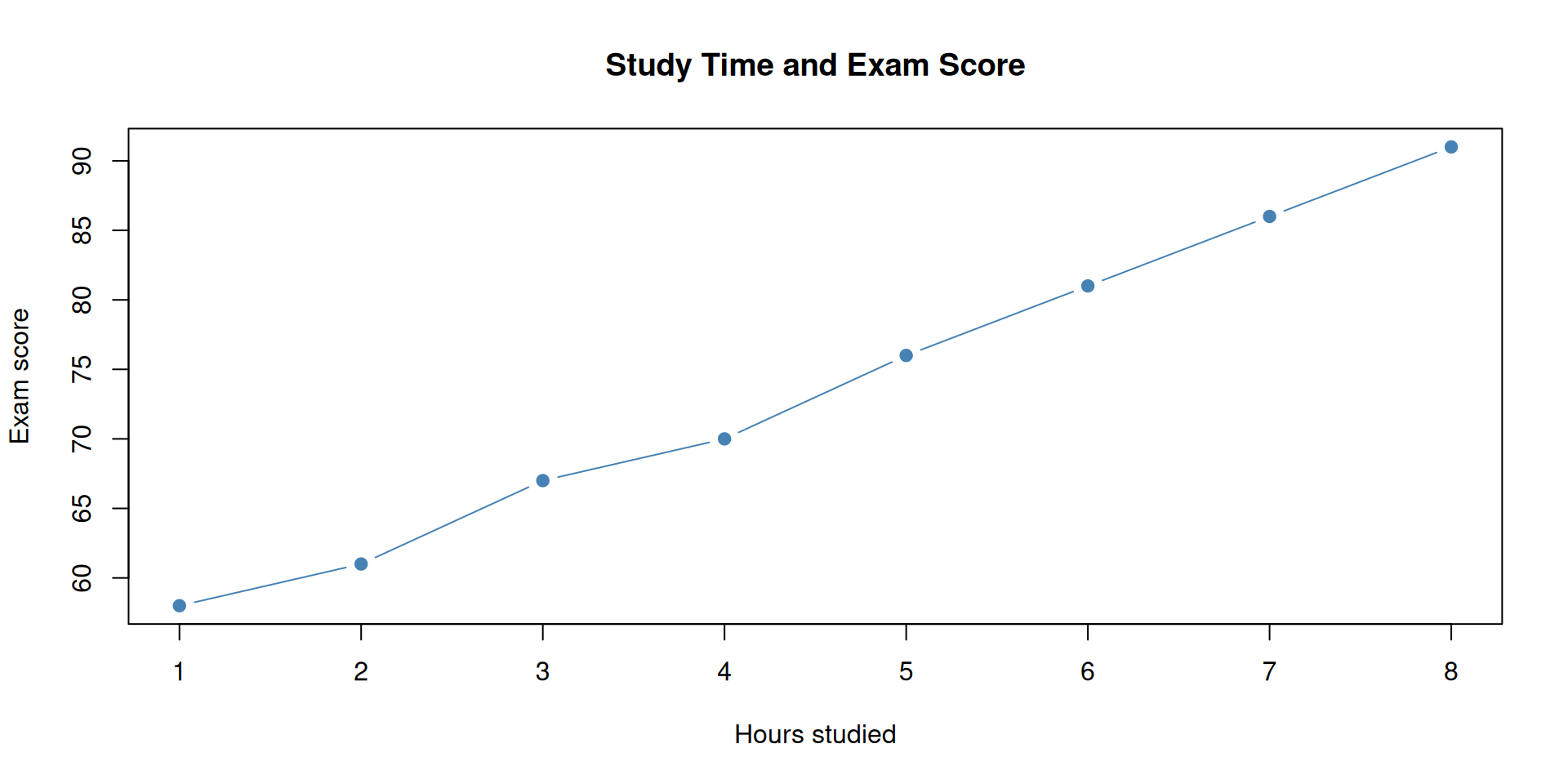
Use plot(x, y) to place one numeric variable on the horizontal axis and another on the vertical axis. Add a title, labels, colors, and point styles to make the graph easier to read.

# Create synthetic data for a small class experiment
study_data <- data.frame(
  hours_studied = c(1, 2, 3, 4, 5, 6, 7, 8),
  exam_score = c(58, 61, 67, 70, 76, 81, 86, 91)
)

# Plot one column against another
plot(study_data$hours_studied, study_data$exam_score,
     main = "Study Time and Exam Score",
     xlab = "Hours studied",
     ylab = "Exam score",
     pch = 19,
     col = "steelblue")

# Add a fitted trend line to highlight the relationship
abline(lm(exam_score ~ hours_studied, data = study_data),
       col = "firebrick", lwd = 2)

Reading a `plot()` Call

plot(
  study_data$hours_studied, # x values
  study_data$exam_score,    # y values
  type = "b",              # points and lines
  pch = 19,                 # point shape
  col = "steelblue",       # color
  main = "Study Time and Exam Score",
  xlab = "Hours studied",
  ylab = "Exam score"
)

Useful plot() options

type = "p" makes points (the default)
type = "l" makes lines
type = "b" makes both points and lines
pch chooses the point shape
col sets the data color
main, xlab, and ylab add readable text

A More Complex Plot with Built-In Data

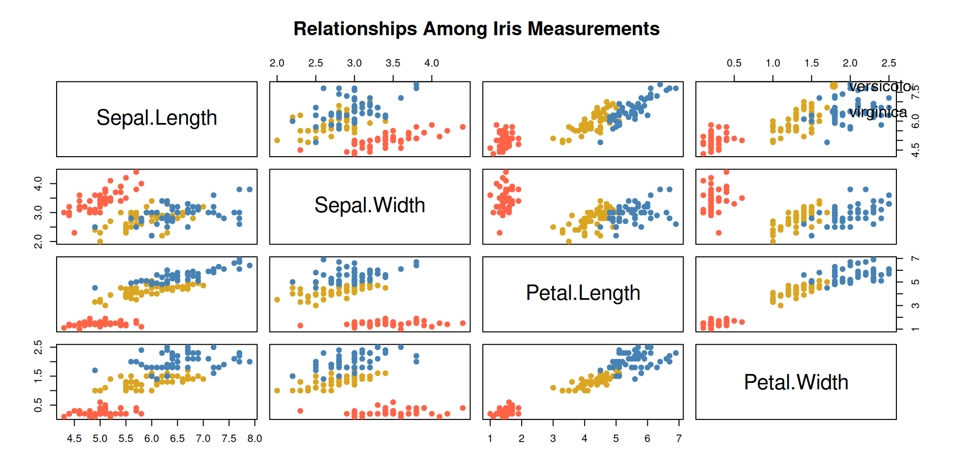
R includes the iris data frame: flower measurements for three species. Passing several numeric columns to plot() creates a scatterplot matrix, so we can compare every measurement against every other one at once.

# One color for each iris species
iris_colors <- c("tomato", "goldenrod", "steelblue")[as.numeric(iris$Species)]

# plot.data.frame() creates a scatterplot matrix for the four measurements
plot(iris[1:4],
     main = "Relationships Among Iris Measurements",
     pch = 19,
     col = iris_colors)

legend("topright",
       legend = levels(iris$Species),
       col = c("tomato", "goldenrod", "steelblue"),
       pch = 19,
       bty = "n")

A More Complex Plot with Built-In Data (Output)

Interactive: `plot()` Code Generator

Build a Base R Plot

Data

X-axis data

Y-axis data

Plot type

Title

X-axis label

Y-axis label

Color

Point shape

Choose options and select "Generate Code".

It’s Time for Some Light Research!!

SunSpots Dataset Analysis

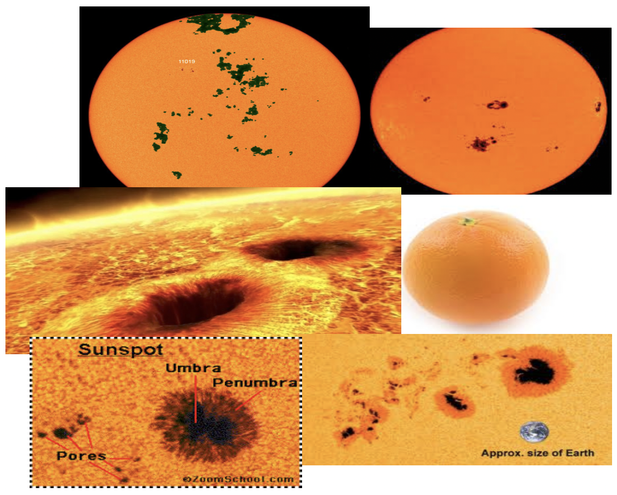
We are going to analyze a dataset called Sunspots which contains monthly sunspot numbers from 1749 to 1983. This dataset is built into R and is a classic example of time series data. We’ll explore its structure, visualize the data, and perform some basic time series analysis.

Articulating the Research Question

Important

Is there a pattern of any kind in this data?
Is there something periodic about the sunspot data?
Can we collect come evidence of a pattern in the data?
Could we use this pattern to predict?
What does a pattern look like in the data?

Sunspots Analysis Code



rm(list = ls()) # clear out the variables from memory to make a clean execution of the code.

# If you want to remove all previous plots and clear the console, run the following two lines.
graphics.off() # clear out all plots from previous work.

cat("\014") # clear the console


if(!require('tidyverse')) {
  install.packages('tidyverse')
  library('tidyverse')
}


# Load the built-in sunspots dataset (monthly data from 1749 to 1983)
data(sunspots)

# 1. View basic information about the time series
print(start(sunspots))  # Start year/month
print(end(sunspots))    # End year/month
print(frequency(sunspots)) # 12 observations per year (monthly)

# 2. Plot the full time series
plot(sunspots, 
     main = "Monthly Sunspot Numbers (1749–1983)", 
     ylab = "Number of Sunspots", 
     xlab = "Year", 
     col = "blue")

# 3. Subset a smaller window to clearly see the 11-year solar cycle
# Let's look at 10 cycles from 1870 to 1970
sunspots_subset <- window(sunspots, start = c(1870, 1), end = c(1970, 12))

plot(sunspots_subset, 
     main = "Sunspot Cycles (1870–1970)", 
     ylab = "Sunspot Count", 
     xlab = "Year", 
     col = "darkred")

# 4. Decompose the time series into trend, seasonal, and random components
# Using additive decomposition (frequency = 12)
sunspots_decomp <- decompose(sunspots_subset)
plot(sunspots_decomp)

# 5. Fit a simple Holt-Winters exponential smoothing or autoregressive model
# (Requires forecast package, or use base AR: ar(sunspots_subset))
fit <- ar(sunspots_subset)
print(fit$order) # Shows the optimal autoregressive lag order

Activity by Month Visualization



# Convert the time series to a data frame for custom ggplot grouping
df <- data.frame(
  Year = as.numeric(time(sunspots_subset)),
  Month = factor(cycle(sunspots_subset), labels = month.abb),
  Count = as.numeric(sunspots_subset)
)

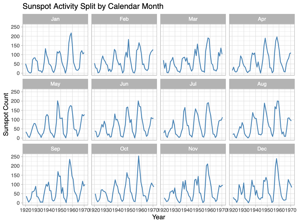
# We will use a new way to visualize the data by month using ggplot2.
# This will allow us to see the sunspot activity for each calendar
# month across the years.

ggplot(df, aes(x = Year, y = Count)) +
  geom_line(color = "steelblue") +
  facet_wrap(~ Month, ncol = 4) +
  labs(title = "Sunspot Activity Split by Calendar Month",
       x = "Year",
       y = "Sunspot Count") +
  theme_light()

Month Visualization Output

Activity by Year Visualization


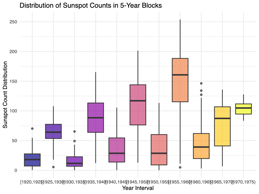
# Create 5-year groupings to see macro-cycles
df$YearGroup <- cut(df$Year, breaks = seq(1920, 1975, by = 5), right = FALSE)

ggplot(df, aes(x = YearGroup, y = Count, fill = YearGroup)) +
  geom_boxplot(alpha = 0.7, show.legend = FALSE) +
  scale_fill_viridis_d(option = "plasma") +
  labs(title = "Distribution of Sunspot Counts in 5-Year Blocks",
       x = "Year Interval",
       y = "Sunspot Count Distribution") +
  theme_minimal()

Year Visualization Output

Observations and Further Analyses?

Observation: The data reveals a distinct 11-year solar cycle, with peaks in sunspot activity occurring approximately every 11 years. The activity is not evenly distributed across the years, with some periods showing higher activity than others.

Important

Further Analyses: Does your analysis of the sunspot data reveal any other patterns or cycles? How might these patterns be useful for predicting future sunspot activity or understanding solar phenomena?

Tip

Even Further Analyses: Remember that this is just a simplified analysis. More advanced time series techniques (like ARIMA modeling, spectral analysis, or machine learning approaches) could provide deeper insights into the sunspot data and its predictive capabilities.

Recap & Up Next

From Today

✅ Lists — Flexible containers for mixed data
✅ Matrices — 2D numeric arrays
✅ Data Frames — The heart of R data analysis
✅ Reading CSV files
✅ Interactive tools for building data structures
✅ Basic plotting with plot()
✅ Some experience with ggplot2 (more coming soon)

Up Next: Data Manipulation with dplyr

📚 Practice: Create data frames, explore built-in datasets
💻 Install: install.packages("tidyverse")
🔮 Preview: We’ll learn the powerful dplyr verbs for data wrangling!

R Fundamentals Part 2

What’s on for today?

Quick Recap: Vectors

Part 1: Lists - The Flexible Container

What Are Lists?

Interactive: List Builder

🔧 Interactive List Creator

Part 2: Matrices - 2D Numeric Data

Creating Matrices

Matrix Operations

Accessing Matrix Elements

Interactive: Matrix Builder 🎮

🎯 Matrix Creator & Visualizer

Part 3: Data Frames - The Star of R!

What Are Data Frames?

Why Data Frames Are Amazing

Interactive: Data Frame Creator

📊 Build Your Own Data Frame!

Part 4: Reading Data Files

Reading CSV Files

Built-in Datasets in R

Quick Challenges!

Challenge 1: Data Frame Access

Challenge 2: Matrix Dimensions

Challenge 3: List vs Data Frame

Challenge 4: Code Writing

Comparing Data Structures

Quick Reference: Data Structures

Visualizing Data with plot()

Reading a plot() Call

A More Complex Plot with Built-In Data

A More Complex Plot with Built-In Data (Output)

Interactive: plot() Code Generator

Build a Base R Plot

It’s Time for Some Light Research!!

SunSpots Dataset Analysis

Articulating the Research Question

Sunspots Analysis Code

Activity by Month Visualization

Month Visualization Output

Activity by Year Visualization

Year Visualization Output

Observations and Further Analyses?

Recap & Up Next

Visualizing Data with `plot()`

Reading a `plot()` Call

Interactive: `plot()` Code Generator