Data Manipulation & Cleaning Part 1

Mastering dplyr for Data Wrangling

What’s on for today?

Today’s Mission: Data Wrangling

📦 Tidyverse — The modern R ecosystem
🔀 The Pipe — %>% operator for readable code
🔧 dplyr Verbs — select, filter, mutate, arrange, summarize

Transform messy data into insights!

The Tidyverse Revolution

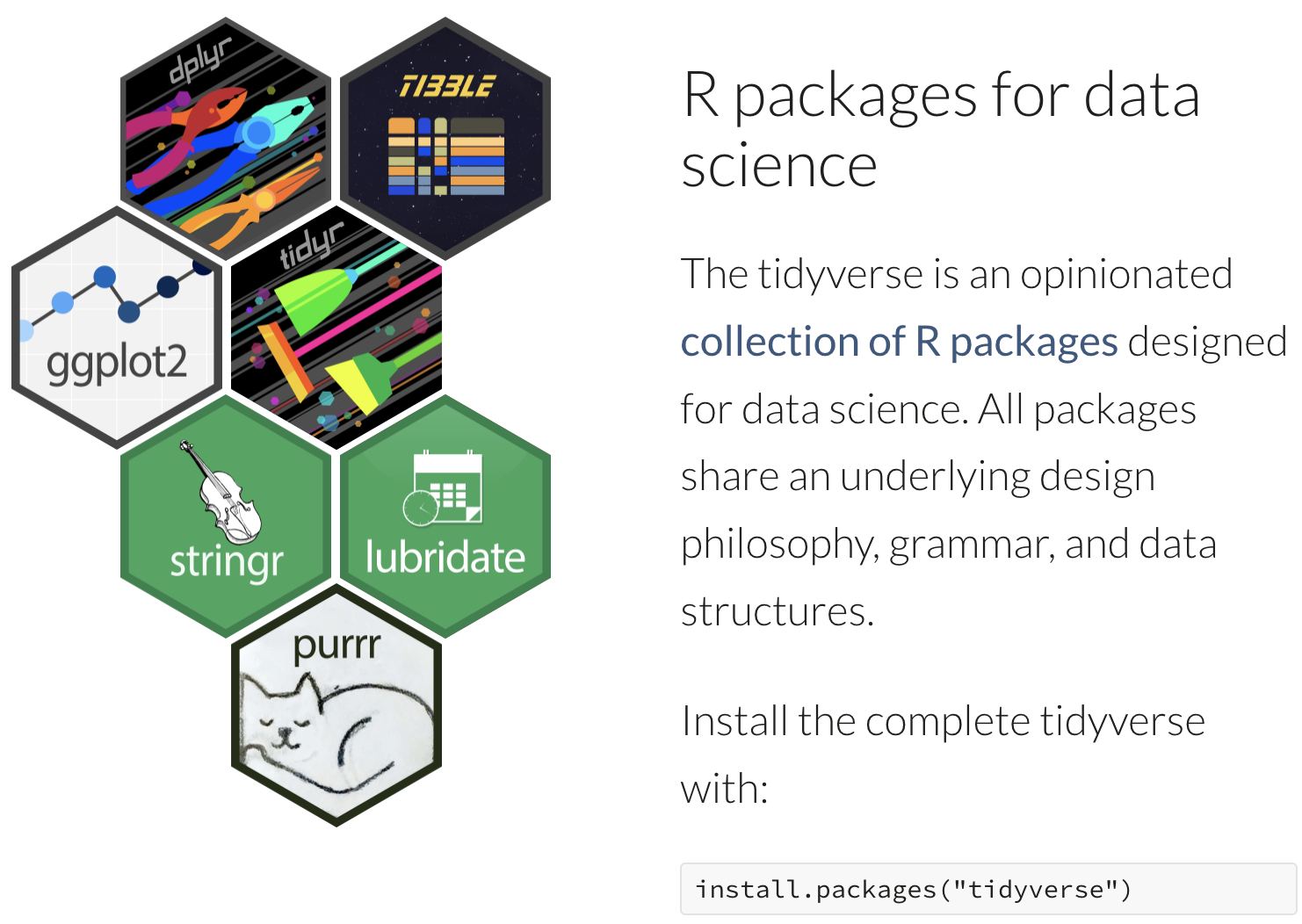
What is the Tidyverse?

Tidyverse: R’s Modern Data Science Toolkit

A collection of packages designed to work together seamlessly!

# Install once
install.packages("tidyverse")

# Load in every session
library(tidyverse)

# You get a buncha packages!
# ✅ dplyr    — Data manipulation
# ✅ ggplot2  — Visualization
# ✅ tidyr    — Data tidying
# ✅ readr    — Reading data
# ✅ purrr    — Functional programming
# ✅ tibble   — Modern data frames
# ✅ stringr  — String manipulation
# ✅ forcats  — Factor handling

But First This!

The Pipe Operators: `%>%` and `|>`

Make Your Code Read Like a Story!

The pipe %>% (and also written as |>) passes output from one function to the next.

With and Without Pipes

Without Pipes

# Nested (hard to read)
result <- arrange(
            filter(
              select(mtcars, mpg, hp, cyl),
              hp > 100
            ),
            desc(mpg)
          )

# Or many temp variables
temp1 <- select(mtcars, mpg, hp, cyl)
temp2 <- filter(temp1, hp > 100)
result <- arrange(temp2, desc(mpg))

With Pipes

# Clean, readable!
result <- mtcars %>%
  select(mpg, hp, cyl) %>%
  filter(hp > 100) %>%
  arrange(desc(mpg))

# Reads like instructions:
# 1. Take mtcars
# 2. Select these columns
# 3. Keep only hp > 100
# 4. Sort by mpg descending

Keyboard shortcut: Cmd/Ctrl + Shift + M = %>%

Tip

You are not the only person reading your code. Write it readably for humans, not just computers!

Looking for a single book in many?

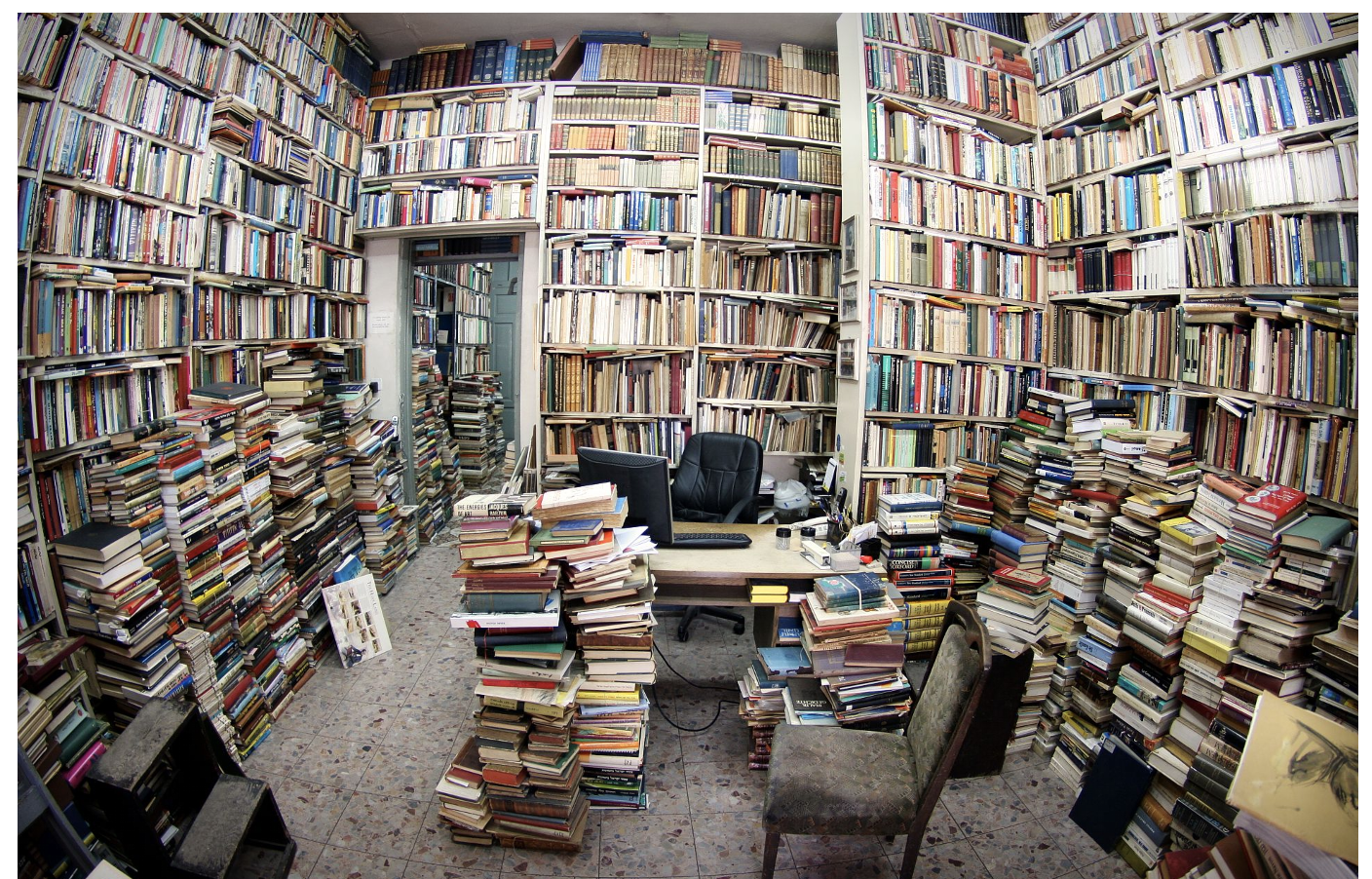
Imagine looking for a single book in a messy bookstore. Do you search by genre, author, or title? How to separate the book from the others?

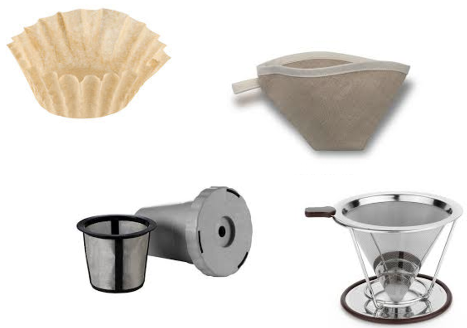
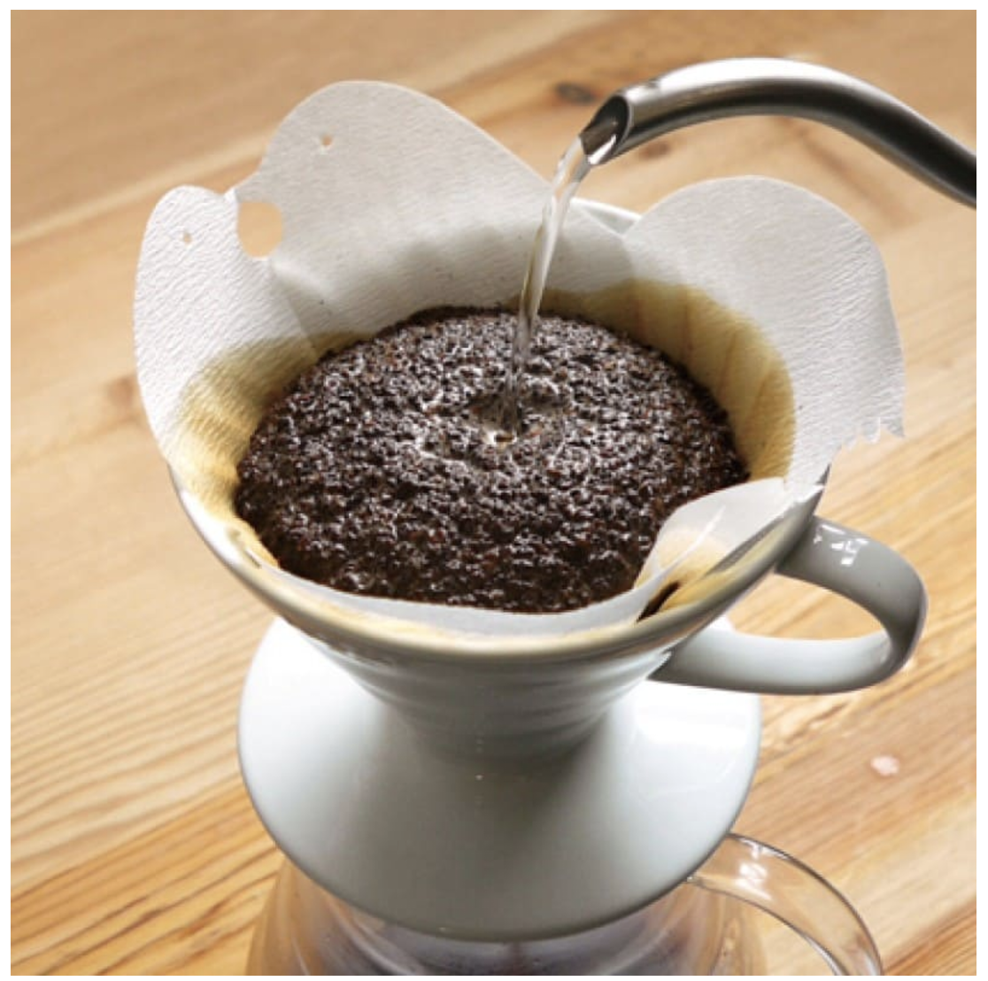
To find things, we can use filters!

Note

Data manipulation is a similar challenge: finding the right information in a messy dataset.

The dplyr Verbs 1

Six powerful functions that solve 90% of data manipulation tasks!

Verb	Purpose	Example
`select()`	Choose columns	`select(data, name, age)`
`filter()`	Choose rows	`filter(data, age > 18)`
`mutate()`	Create/modify columns	`mutate(data, age_squared = age^2)`

The dplyr Verbs 2

Six powerful functions that solve 90% of data manipulation tasks!

Verb	Purpose	Example
`arrange()`	Sort rows	`arrange(data, desc(age))`
`summarize()`	Aggregate data	`summarize(data, mean_age = mean(age))`
`group_by()`	Group for operations	`group_by(data, category)`

1. select() — Choose Columns

Pick the columns you need

# Load example data
library(tidyverse)
data(mtcars)

# Select specific columns
mtcars %>% select(mpg, cyl, hp)

# Select range of columns
mtcars %>% select(mpg:hp)

# Select by pattern
mtcars %>% select(starts_with("m"))    # mpg
mtcars %>% select(ends_with("p"))      # hp, disp
mtcars %>% select(contains("ar"))      # gear, carb

# Exclude columns
mtcars %>% select(-wt, -qsec)

# Reorder columns
mtcars %>% select(hp, mpg, everything())

# Rename while selecting
mtcars %>% select(miles_per_gallon = mpg, horsepower = hp)

2. filter() — Choose Rows

Keep only rows that meet conditions

# Simple filter
mtcars %>% filter(mpg > 20)

# Multiple conditions (AND)
mtcars %>% filter(mpg > 20, cyl == 4)
mtcars %>% filter(mpg > 20 & cyl == 4)

# OR conditions
mtcars %>% filter(cyl == 4 | cyl == 6)
mtcars %>% filter(cyl %in% c(4, 6))

# Complex conditions
mtcars %>% filter(
  mpg > 20,
  cyl %in% c(4, 6),
  hp < 100
)

# Pattern matching
library(datasets)
data(iris)
iris %>% filter(grepl("setosa", Species))

# Missing values
data %>% filter(is.na(column))      # Keep NAs
data %>% filter(!is.na(column))     # Remove NAs

3. mutate() — Create/Modify Columns

Add or change variables

# Create new column
mtcars %>% 
  mutate(hp_per_cyl = hp / cyl)

# Multiple new columns
mtcars %>%
  mutate(
    kml = mpg * 0.425,           # Convert to km/L
    hp_per_cyl = hp / cyl,
    is_powerful = hp > 150
  )

# Use newly created columns
mtcars %>%
  mutate(
    hp_per_cyl = hp / cyl,
    rating = ifelse(hp_per_cyl > 50, "High", "Low")
  )

# Modify existing column
mtcars %>%
  mutate(mpg = round(mpg, 0))

# Conditional mutation
mtcars %>%
  mutate(
    efficiency = case_when(
      mpg > 25 ~ "High",
      mpg > 20 ~ "Medium",
      TRUE ~ "Low"
    )
  )

4. arrange() — Sort Rows

Order your data

# Sort ascending (default)
mtcars %>% arrange(mpg)

# Sort descending
mtcars %>% arrange(desc(mpg))

# Multiple columns
mtcars %>% arrange(cyl, desc(mpg))

# Useful with other verbs
mtcars %>%
  filter(hp > 100) %>%
  select(mpg, hp, cyl) %>%
  arrange(desc(mpg))

# Top N
mtcars %>%
  arrange(desc(mpg)) %>%
  head(5)  # Top 5 most efficient

# Bottom N
mtcars %>%
  arrange(mpg) %>%
  head(5)  # 5 least efficient

5. summarize() — Aggregate Data

Calculate summary statistics

# Single summary
mtcars %>%
  summarize(mean_mpg = mean(mpg))

# Multiple summaries
mtcars %>%
  summarize(
    avg_mpg = mean(mpg),
    sd_mpg = sd(mpg),
    min_mpg = min(mpg),
    max_mpg = max(mpg),
    count = n()
  )

# Useful functions in summarize()
data %>%
  summarize(
    mean = mean(x),
    median = median(x),
    sd = sd(x),
    min = min(x),
    max = max(x),
    sum = sum(x),
    n = n(),                    # Count rows
    n_distinct = n_distinct(x)  # Count unique values
  )

6. group_by() — Group Operations

The Game Changer!

group_by() + summarize() = Super powerful analysis

# Group by cylinder and summarize
mtcars %>%
  group_by(cyl) %>%
  summarize(
    count = n(),
    avg_mpg = mean(mpg),
    avg_hp = mean(hp)
  )
#   cyl count avg_mpg avg_hp
#   4      11    26.7   82.6
#   6       7    19.7  122.3
#   8      14    15.1  209.2

# Multiple grouping variables
mtcars %>%
  group_by(cyl, gear) %>%
  summarize(avg_mpg = mean(mpg))

# Group + mutate (add group stats to each row)
mtcars %>%
  group_by(cyl) %>%
  mutate(
    mean_mpg_by_cyl = mean(mpg),
    diff_from_mean = mpg - mean_mpg_by_cyl
  )

Interactive: dplyr Pipeline Builder

🔧 Build Your dplyr Pipeline!

Dataset:

Example: mpg, cyl, hp

Build your pipeline and click "Generate Code"!

Quick Challenges!

Challenge 1: Pipe Order

What's the correct order for: "Filter cars with mpg > 20, then select cyl and mpg"?

select(cyl, mpg) |> filter(mpg > 20)

filter(mpg > 20) |> select(cyl, mpg)

Both work the same

group_by(mpg) |> filter(mpg > 20)

Challenge 2: Mutate vs Summarize

Which creates a NEW column while keeping all rows?

mutate()

summarize()

filter()

arrange()

Challenge 3: Filter Conditions

Which command keeps cars with 6 or 8 cylinders?

filter(cyl == 6 & cyl == 8)

filter(cyl == 6 | cyl == 8)

select(cyl == 6 | cyl == 8)

arrange(cyl == 6 | cyl == 8)

Challenge 4: Sorting Rows

Which pipeline puts the most powerful cars first?

mtcars |> arrange(hp)

mtcars |> arrange(desc(hp))

mtcars |> filter(desc(hp))

mtcars |> summarize(desc(hp))

Challenge 5: Grouped Summaries

Which pipeline finds average mpg for each number of cylinders?

mtcars |> summarize(avg_mpg = mean(mpg)) |> group_by(cyl)

mtcars |> group_by(cyl) |> summarize(avg_mpg = mean(mpg))

mtcars |> mutate(avg_mpg = mean(mpg), cyl)

mtcars |> select(cyl, mean(mpg))

Programming Challenges

Note

Work with a partner first. Write each pipeline before checking the following solution slides.

Challenge 6: Select and Filter

Using mtcars, create a table with only mpg, hp, and wt for cars with more than 150 horsepower using commands, use select() and filter(). Use arrange() with argument desc(wt) to put the heaviest cars first.

Challenge 6: Solution

mtcars |>
  select(mpg, hp, wt) |> % and then
  filter(hp > 150) |> %and then
  arrange(desc(wt))

Challenge 7: Create a Useful Column

Using mtcars, add a column named power_per_weight equal to horsepower divided by weight. Keep only cars with power_per_weight greater than 50, then show mpg, hp, wt, and the new column.

Challenge 7: Solution

mtcars |>
  mutate(power_per_weight = hp / wt) |>
  filter(power_per_weight > 50) |>
  select(mpg, hp, wt, power_per_weight)

Challenge 8: Summarize by Group

Using iris, calculate the number of flowers and the average petal length for each species. Sort the result from the largest average petal length to the smallest.

Challenge 8: Solution

iris |>
  group_by(Species) |>
  summarize(
    flower_count = n(),
    average_petal_length = mean(Petal.Length)
  ) |>
  arrange(desc(average_petal_length))

Data Manipulation & Cleaning Part 1

What’s on for today?

The Tidyverse Revolution

What is the Tidyverse?

But First This!

The Pipe Operators: %>% and |>

With and Without Pipes

Looking for a single book in many?

To find things, we can use filters!

The dplyr Verbs 1

The dplyr Verbs 2

1. select() — Choose Columns

2. filter() — Choose Rows

3. mutate() — Create/Modify Columns

4. arrange() — Sort Rows

5. summarize() — Aggregate Data

6. group_by() — Group Operations

Interactive: dplyr Pipeline Builder

🔧 Build Your dplyr Pipeline!

Quick Challenges!

Challenge 1: Pipe Order

Challenge 2: Mutate vs Summarize

Challenge 3: Filter Conditions

Challenge 4: Sorting Rows

Challenge 5: Grouped Summaries

Programming Challenges

Challenge 6: Select and Filter

Challenge 6: Solution

Challenge 7: Create a Useful Column

Challenge 7: Solution

Challenge 8: Summarize by Group

Challenge 8: Solution

The Pipe Operators: `%>%` and `|>`