Confidence Concepts

Statistical Inference: confidence intervals

Up for Today

From Description to Inference

  • Confidence Intervals โ€” putting error bars on everything

Confidence Intervals ๐Ÿ“

What 95% Confidence Actually Means (Visually)

library(tidyverse)

set.seed(301)

# Build 100 confidence intervals from 100 different samples
cis <- map_dfr(1:100, function(i) {
  s  <- rnorm(30, mean = 170, sd = 10)
  tt <- t.test(s)
  tibble(trial = i, est = mean(s),
         lower = tt$conf.int[1], upper = tt$conf.int[2])
}) %>%
  mutate(captures = lower <= 170 & upper >= 170)

cat("Intervals containing the true mean:", sum(cis$captures), "out of 100\n")
Intervals containing the true mean: 95 out of 100
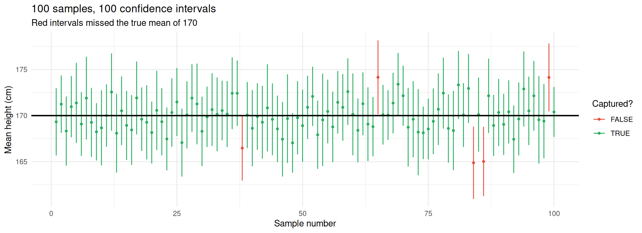
What 95% ConfidenceActually Means Visually Plot

ggplot(cis, aes(trial, est, color = captures)) +
  geom_errorbar(aes(ymin = lower, ymax = upper), width = 0) +
  geom_point(size = 1) +
  geom_hline(yintercept = 170, color = "black", linewidth = 0.8) +
  scale_color_manual(values = c("FALSE" = "#E74C3C", "TRUE" = "#27AE60")) +
  labs(title = "100 samples, 100 confidence intervals",
       subtitle = "Red intervals missed the true mean of 170",
       x = "Sample number", y = "Mean height (cm)", color = "Captured?") +
  theme_minimal(base_size = 11)

95% confidence means that if we were to repeat this process many times, about 95% of the resulting confidence intervals would contain the true mean. Here, five of the 100 confidence intervals missed the true mean of 170.

What a Confidence Interval Is

Important

A 95% CI is a range built by a procedure that captures the true parameter 95% of the time in repeated sampling.

Letโ€™s Try It Out

We calculate a 95% confidence interval for the population mean height using a random sample of 30 people. It uses the t-distribution because the population standard deviation is unknown and is estimated using the sample data.

Calculating a confidence interval is a four-step process:

  • Compute the sample mean and standard error.
  • Find the critical value from the t-distribution (or z-distribution if sigma is known).
  • Compute the margin of error.
  • Construct the interval: mean ยฑ margin of error.

Code to compute a 95% confidence interval for the mean height from a random sample of 30 people

set.seed(301)

# Generate a random sample of 30 heights (in cm) from a normal distribution
heights <- rnorm(30, mean = 170, sd = 10)   # one random normal sample

# Compute the sample mean and standard error
# heights refers to the 30 simulated observations
x_bar <- mean(heights) # avg of 30 sample means
s     <- sd(heights) # sample standard deviation
n     <- length(heights) # Find the sample size
se    <- s / sqrt(n) # Find the standard error of the mean

# Note: The standard error estimates how much the
# sample mean would vary across repeated random samples
# of the same size.

# Find the critical value from the t-distribution.
# The sigma value is unknown, so we use the 
# t-distribution with n-1 degrees of freedom
# How to find the critical value? For a 95%
# confidence level, we want the value that leaves 2.5% in each tail.

t_crit <- qt(0.975, df = n - 1)

# We calculate the lower and upper bounds of the 95%
# confidence interval
# The interval provides a range of plausible values for the
# population mean, based on the sample data and the assumptions 
# of the t-interval method.
ci <- c(x_bar - t_crit * se, x_bar + t_crit * se)
round(c(mean = x_bar, se = se, lower = ci[1], upper = ci[2]), 2)
  mean     se  lower  upper 
169.33   1.78 165.68 172.97 

Tip

The standard error (se) estimates how much the sample mean would vary across repeated random samples of the same size.

How to make Sense of a Confidence Interval

Some ideas about confidence intervals

  • Purpose: A confidence interval estimates a plausible range for the unknown population mean height.

  • A 95% confidence interval means that if we were to repeat this process many times, about 95% of the resulting confidence intervals would contain the true mean. Here, five of the 100 confidence intervals missed the true mean of 170.

  • Confidence level: A 95% confidence interval is produced by using the 0.975 quantile of the t-distribution.

Important

  • Interpretation: If we repeatedly collected samples of 30 people and calculated a confidence interval in the same way, approximately 95% of those intervals would contain the true population mean, assuming the modelโ€™s conditions hold.

The One-Line Version to Compute Confidence Intervals

# t.test() computes the same interval at 95% confidence level by default
t.test(heights)$conf.int
[1] 165.6761 172.9745
attr(,"conf.level")
[1] 0.95
# Change the confidence level to 99% using the conf.level argument
t.test(heights, conf.level = 0.99)$conf.int
[1] 164.4073 174.2433
attr(,"conf.level")
[1] 0.99
# CI for a proportion: 42 successes out of 100 trials
prop.test(42, 100)$conf.int
[1] 0.3233236 0.5228954
attr(,"conf.level")
[1] 0.95

Tip

Wider confidence = wider interval. A 99% CI is more likely to be right and less informative. A measure of certainty of the estimate is traded off against precision of the estimate.

The Interpretation Trap ๐Ÿชค

โŒ Wrong

โ€œThere is a 95% probability that ฮผ is between 167 and 173.โ€

The true ฮผ is a fixed number. It is either in your interval or it is not โ€” no probability involved. ๐ŸŽฒ

โœ… Right

โ€œWe are 95% confidentโ€ฆโ€ meaning: this method produces intervals that capture ฮผ 95% of the time.

The randomness lives in the interval, not in ฮผ.

The Practical Reading

A CI tells you which values are compatible with your data. If a claimed value falls outside your interval, your data argues against it. ๐Ÿ“Š

Interactive: Confidence Interval Calculator ๐ŸŽฎ

๐Ÿ“ Confidence Interval Calculator

Choose what you are estimating and click "Generate Code"!

Knowledge Check ๐Ÿง 

You quadruple your sample size from 100 to 400. What happens to the width of your confidence interval?
It shrinks to one quarter of its width
It shrinks to about half its width
It stays the same โ€” the confidence level did not change
It doubles

Quick Challenges! ๐Ÿง 

Challenge 1: Picking the Prefix

A factory's bolts have length ~ Normal(50mm, 0.4mm). You need the proportion that fall outside 49mm-51mm (the reject rate). Which expression is right?
dnorm(51, 50, 0.4) - dnorm(49, 50, 0.4)
1 - (pnorm(51, 50, 0.4) - pnorm(49, 50, 0.4))
qnorm(51, 50, 0.4) + qnorm(49, 50, 0.4)
mean(rnorm(1000, 50, 0.4) > 51)

Challenge 2: CLT Limits

Your data is strongly right-skewed with n = 45. Which statement is true?
The CLT makes your data normally distributed
You cannot compute a confidence interval on skewed data
A CI for the MEAN is reasonable, but the mean may not be the statistic you want to report
n = 45 guarantees the sampling distribution is exactly normal

Challenge 3: Reading an Interval

A study reports a 95% CI for a treatment effect of [-0.5, 8.2] points. What is the best summary?
The treatment definitely does not work
The treatment works, with an effect of 3.85 points
The data is compatible with anything from a tiny harm to a large benefit โ€” the study is inconclusive
There is a 95% chance the effect is 3.85 points

Challenge 4: Write the Code

Write code that simulates rolling five dice 10,000 times, and estimates the probability that the total is 20 or more. Then compare your simulation to a normal approximation.

Cheat Sheet (This Weekโ€™s Most Useful Commands)

Note

Task Code
Random sample sample(x, n, replace = TRUE)
Reproducibility set.seed(301)
Density / mass dnorm(), dbinom(), dpois()
P(X โ‰ค q) pnorm(q, mean, sd)
P(X > q) pnorm(q, ..., lower.tail = FALSE)
Quantile qnorm(p, mean, sd)
Random draws rnorm(n, mean, sd)
Repeat a simulation replicate(n, expr)
Standard error sd(x) / sqrt(length(x))
CI for a mean t.test(x)$conf.int
CI for a proportion prop.test(successes, n)$conf.int
t critical value qt(0.975, df = n - 1)