Enter your name :
Your name is :
t-tests & the Truth About p-values
Tip
Some Helpful Stuff …
Formal Statistical Inference
A p-value answers one narrow question. Know exactly which one.
Enter your name :
Your name is :
Getting user input in R
Note
Note: The readline() function is used to get input from the user. It will pause the execution of the code and wait for the user to enter a value. Generally not used in R Markdown documents or on back-end servers, but useful in interactive R scripts.
countDown : 0
countDown : 1
countDown : 2
countDown : 3
countDown : 4
countDown : 5
countDown : 6
countDown : 7
countDown : 8
countDown : 9
countDown : 10
Blast Off!

How we write functions in R
Important
function() keyword is used to define a function, and the function body contains the code that will be executed when the function is called.return() statement is optional; if omitted, the function will return the last evaluated expression.7
Important
return() statement is used to specify the output of the function.return() statement is provided, the function will return the last evaluated expression.# calculating sine of an angle in degrees
sine_degrees <- function(angle_degrees) {
# Convert degrees to radians
angle_radians <- angle_degrees * (pi / 180)
# Calculate sine
sine_value <- sin(angle_radians)
# Return the sine value
return(sine_value)
}
# call the function
cat(sine_degrees(30)) # Output: 0.50.5
# calculating sine of an angle in degrees
sine_degrees <- function(angle_degrees) {
# Convert degrees to radians
angle_radians <- angle_degrees * (pi / 180)
# Calculate sine
sine_value <- sin(angle_radians)
# Return the sine value
return(sine_value)
}
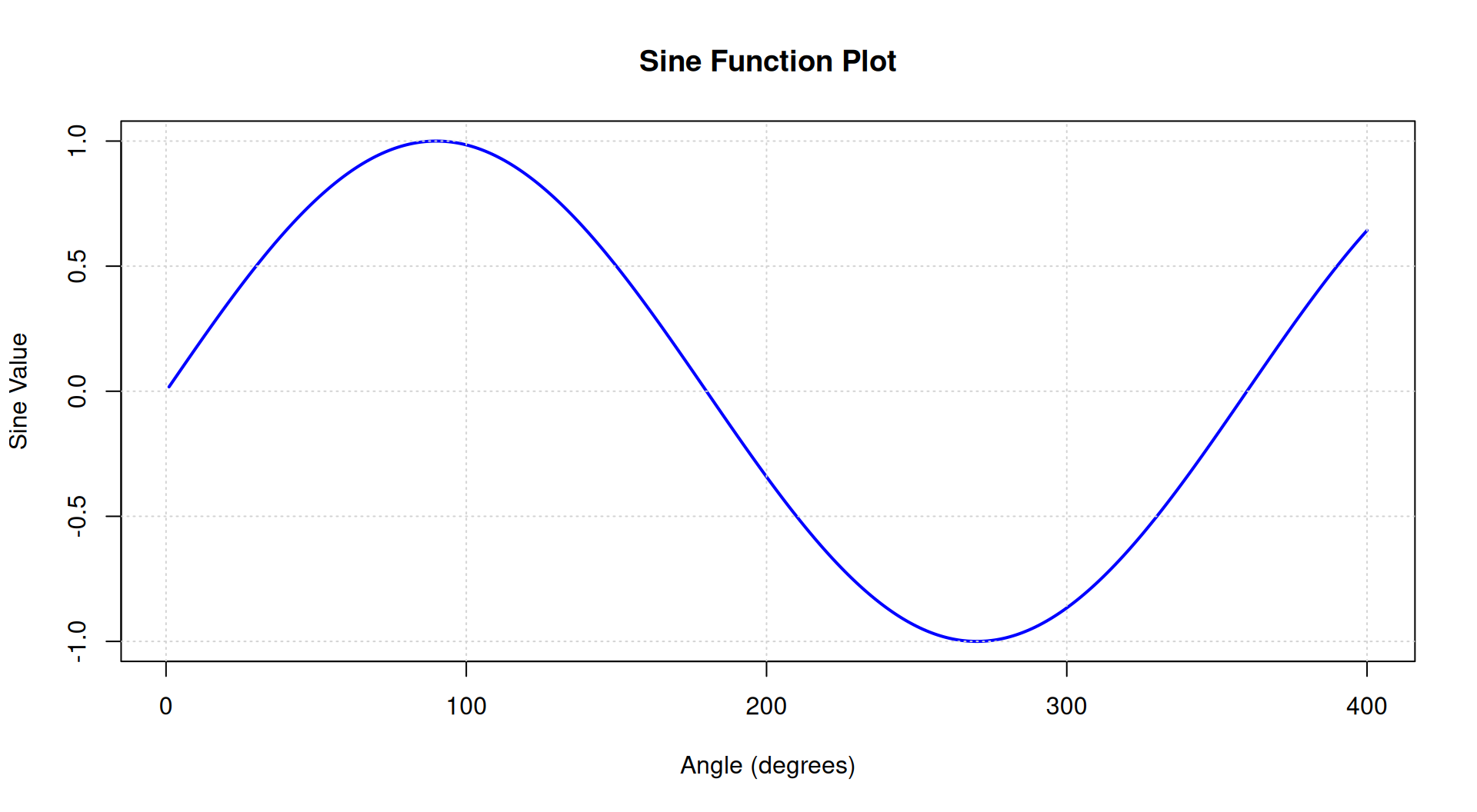
plot_sine <- function(start, end, step) {
# Generate a sequence of angles in degrees
angles <- seq(start, end, by = step)
# Calculate sine values for each angle
sine_values <- sapply(angles, sine_degrees)
# Create the plot
plot(angles, sine_values, type = "l", col = "blue", lwd = 2,
xlab = "Angle (degrees)", ylab = "Sine Value",
main = "Sine Function Plot")
grid() # Add grid lines for better visualization
}
plot_sine(1,400,1)
Tip
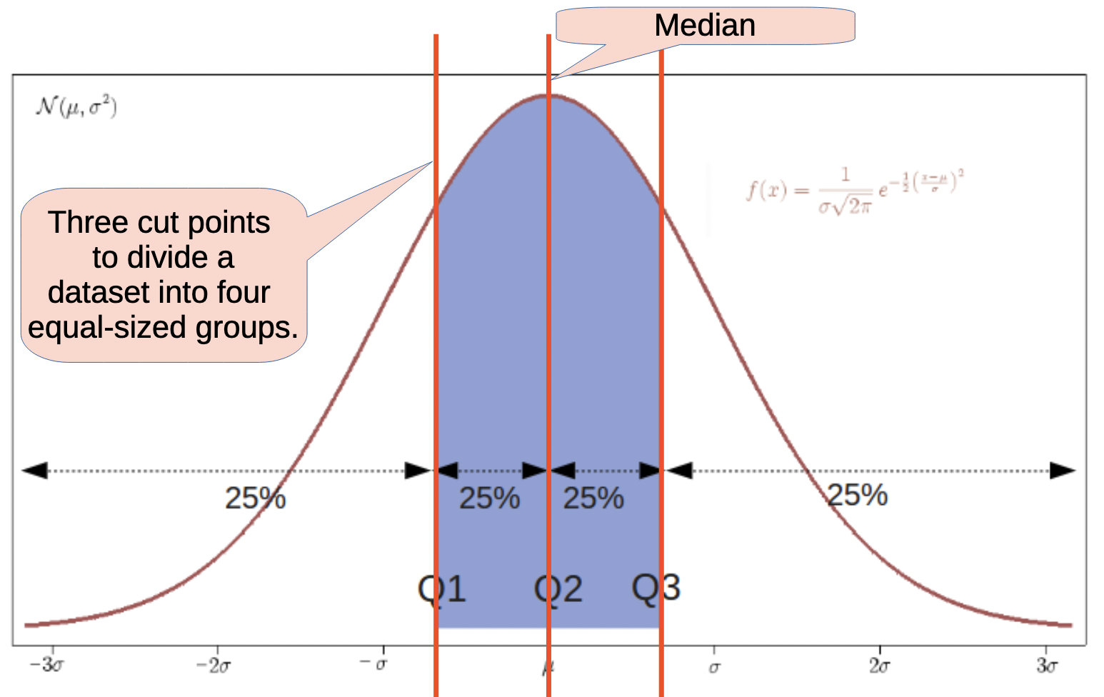
25% 50% 75%
-0.56422487 -0.01148396 0.50636497
Min. 1st Qu. Median Mean 3rd Qu. Max.
-2.85719 -0.56422 -0.01148 -0.07634 0.50636 2.00706
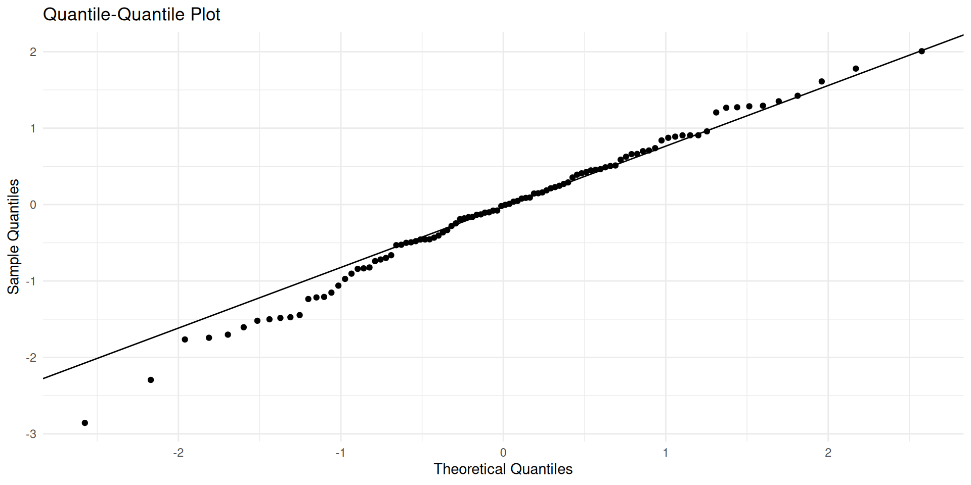
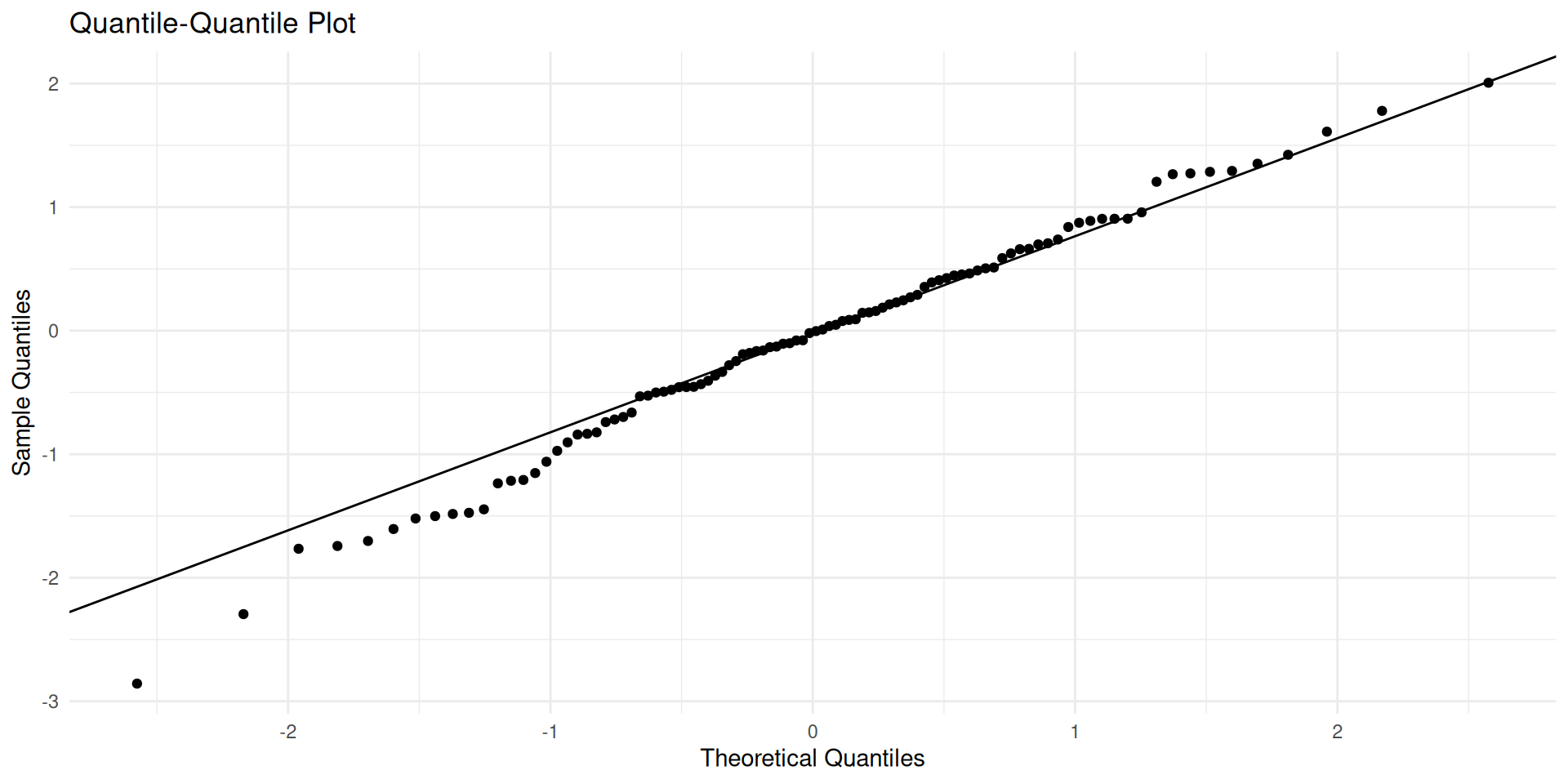
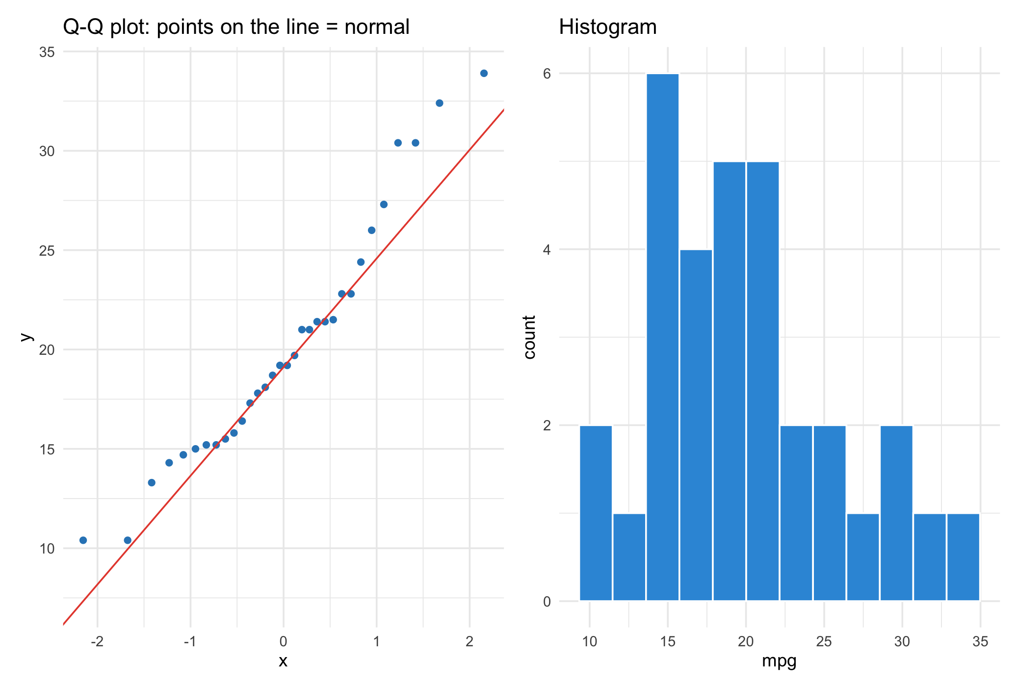
If your data is normally distributed, the points in the Q-Q plot will fall approximately along the reference line. Deviations from this line indicate departures from normality.
library(tidyverse)
# Quartiles
myQuartilePlot <- function(data) {
# Create a data frame for ggplot
df <- data.frame(value = data)
# Create the quantile plot
ggplot(df, aes(sample = value)) +
stat_qq() +
stat_qq_line() +
labs(title = "Quantile-Quantile Plot",
x = "Theoretical Quantiles",
y = "Sample Quantiles") +
theme_minimal()
}
# Generate some sample data
set.seed(301)
data <- rnorm(100)
myQuartilePlot(data)In normal distributions, the points will align with the reference line.
Important
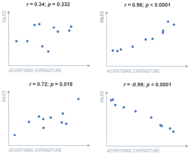
A correlation coefficient measures the strength and direction of the linear relationship between two continuous variables.
Correlation coefficients range from -1 (negative) to 1 (positive), with values closer to -1 or 1 indicating stronger relationships.
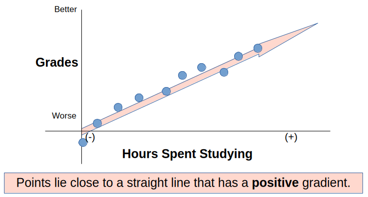
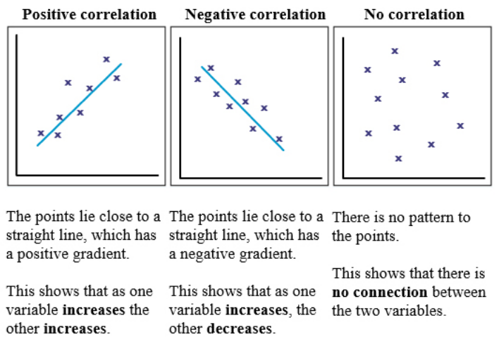
Positive correlation: as one variable increases, the other also increases.
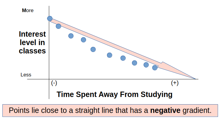
Negative correlation: as one variable increases, the other decreases.
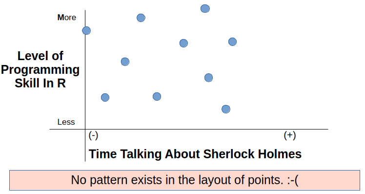
Neutral correlation: the increase in one variable is not related to the increase in the other.
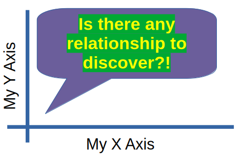
All correlations: positive, negative, and neutral correlations.
Different types of correlation coefficients exist, such as Pearson’s correlation coefficient (for linear relationships) and Spearman’s rank correlation coefficient (for monotonic relationships).
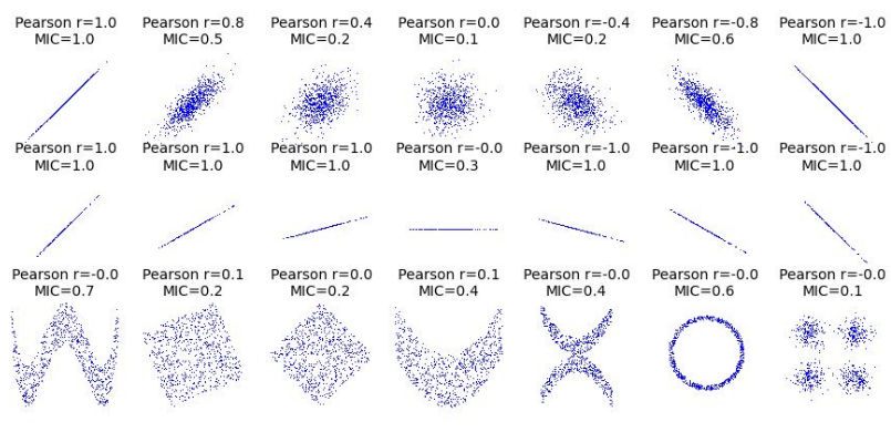
The correlation coefficient is a unitless measure; it does not depend on the units of the variables being measured.
Tip
Correlation measures the strength and direction of the linear relationship between two continuous variables. The correlation coefficient ranges from -1 to 1, where:
[1] 1
[1] -1
GNP.deflator GNP Unemployed Armed.Forces Population
GNP.deflator 1.0000000 0.9915892 0.6206334 0.4647442 0.9791634
GNP 0.9915892 1.0000000 0.6042609 0.4464368 0.9910901
Unemployed 0.6206334 0.6042609 1.0000000 -0.1774206 0.6865515
Armed.Forces 0.4647442 0.4464368 -0.1774206 1.0000000 0.3644163
Population 0.9791634 0.9910901 0.6865515 0.3644163 1.0000000
Year 0.9911492 0.9952735 0.6682566 0.4172451 0.9939528
Employed 0.9708985 0.9835516 0.5024981 0.4573074 0.9603906
Year Employed
GNP.deflator 0.9911492 0.9708985
GNP 0.9952735 0.9835516
Unemployed 0.6682566 0.5024981
Armed.Forces 0.4172451 0.4573074
Population 0.9939528 0.9603906
Year 1.0000000 0.9713295
Employed 0.9713295 1.0000000
GNP.deflator GNP Unemployed Armed.Forces Population
GNP.deflator 1.0000000 0.9915892 0.6206334 0.4647442 0.9791634
GNP 0.9915892 1.0000000 0.6042609 0.4464368 0.9910901
Unemployed 0.6206334 0.6042609 1.0000000 -0.1774206 0.6865515
Armed.Forces 0.4647442 0.4464368 -0.1774206 1.0000000 0.3644163
Population 0.9791634 0.9910901 0.6865515 0.3644163 1.0000000
Year 0.9911492 0.9952735 0.6682566 0.4172451 0.9939528
Employed 0.9708985 0.9835516 0.5024981 0.4573074 0.9603906
Year Employed
GNP.deflator 0.9911492 0.9708985
GNP 0.9952735 0.9835516
Unemployed 0.6682566 0.5024981
Armed.Forces 0.4172451 0.4573074
Population 0.9939528 0.9603906
Year 1.0000000 0.9713295
Employed 0.9713295 1.0000000
GNP. GNP U A P Y E
GNP.deflator 1
GNP B 1
Unemployed , , 1
Armed.Forces . . 1
Population B B , . 1
Year B B , . B 1
Employed B B . . B B 1
attr(,"legend")
[1] 0 ' ' 0.3 '.' 0.6 ',' 0.8 '+' 0.9 '*' 0.95 'B' 1
GNP. GNP U A P Y E
GNP.deflator 1
GNP B 1
Unemployed , , 1
Armed.Forces . . 1
Population B B , . 1
Year B B , . B 1
Employed B B . . B B 1
attr(,"legend")
[1] 0 ' ' 0.3 '.' 0.6 ',' 0.8 '+' 0.9 '*' 0.95 'B' 1
GNP. GNP U A P Y E
GNP.deflator 1
GNP B 1
Unemployed , , 1
Armed.Forces . 1
Population B B , 1
Year B B , 1 1
Employed B B . B B 1
attr(,"legend")
[1] 0 ' ' 0.3 '.' 0.6 ',' 0.8 '+' 0.9 '*' 0.95 'B' 1
GNP. GNP U A P Y E
GNP.deflator 1
GNP B 1
Unemployed . . 1
Armed.Forces 1
Population B B . 1
Year B B . 1 1
Employed * * . + + 1
attr(,"legend")
[1] 0 ' ' 0.3 '.' 0.6 ',' 0.8 '+' 0.9 '*' 0.95 'B' 1
P S K
P 1.0000000 0.9802390 0.9572562
S 0.9802390 1.0000000 0.9742171
K 0.9572562 0.9742171 1.0000000
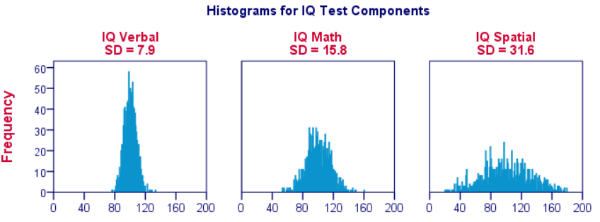
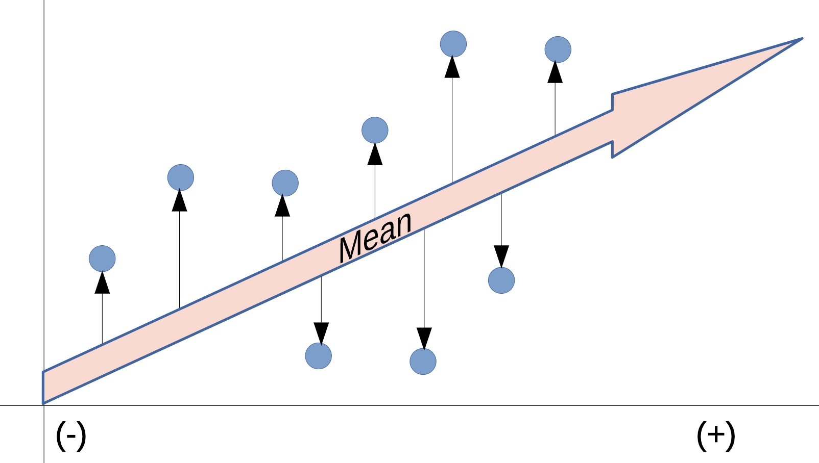
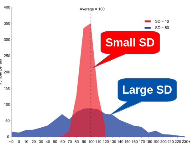
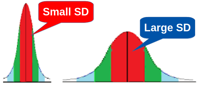
How spread out is the data? Does the data have a lot of variability about the mean?
Variance is a measure of how spread out the data is from the mean. It is calculated by taking the average of the squared differences from the mean.
Tip
Variance is expressed in the squared units of the data, which can make it less interpretable than standard deviation.
The formula for variance (sigma squared) is: \(\sigma^2 = \frac{\sum_{i=1}^{N} (x_i - \mu)^2 }{N}\)
Where,
[1] 9.368421
[1] 3.060788
[1] NA
[1] 9.654971
Standard deviation is the square root of the variance. It is a measure of the amount of variation or dispersion of a set of values.
Tip
If variance is a measure of how spread out the data is, standard deviation is a measure of how much the data deviates from the mean. It is expressed in the same units as the data, making it more interpretable than variance.
The formula for standard deviation (sigma) is: \(\sigma = \sqrt{\frac{\sum_{i=1}^{N} (x_i - \mu)^2 }{N}}\)
Where,

Tip

Tip
Instead of looking for a universal “good” or “bad” number, evaluate your SD using these three methods:
Compare SD to the mean (Coefficient of Variation): Divide the standard deviation by the mean to see relative spread. A lower percentage means your data is tightly clustered around the average.
Compare SD to your requirements or limits.
Compare it over time: Track the number across repeated runs. A rising standard deviation means your process is becoming less stable or predictable.
Above Details stolen indirectly from Wikipedia: https://en.wikipedia.org/wiki/Standard_deviation

Tip
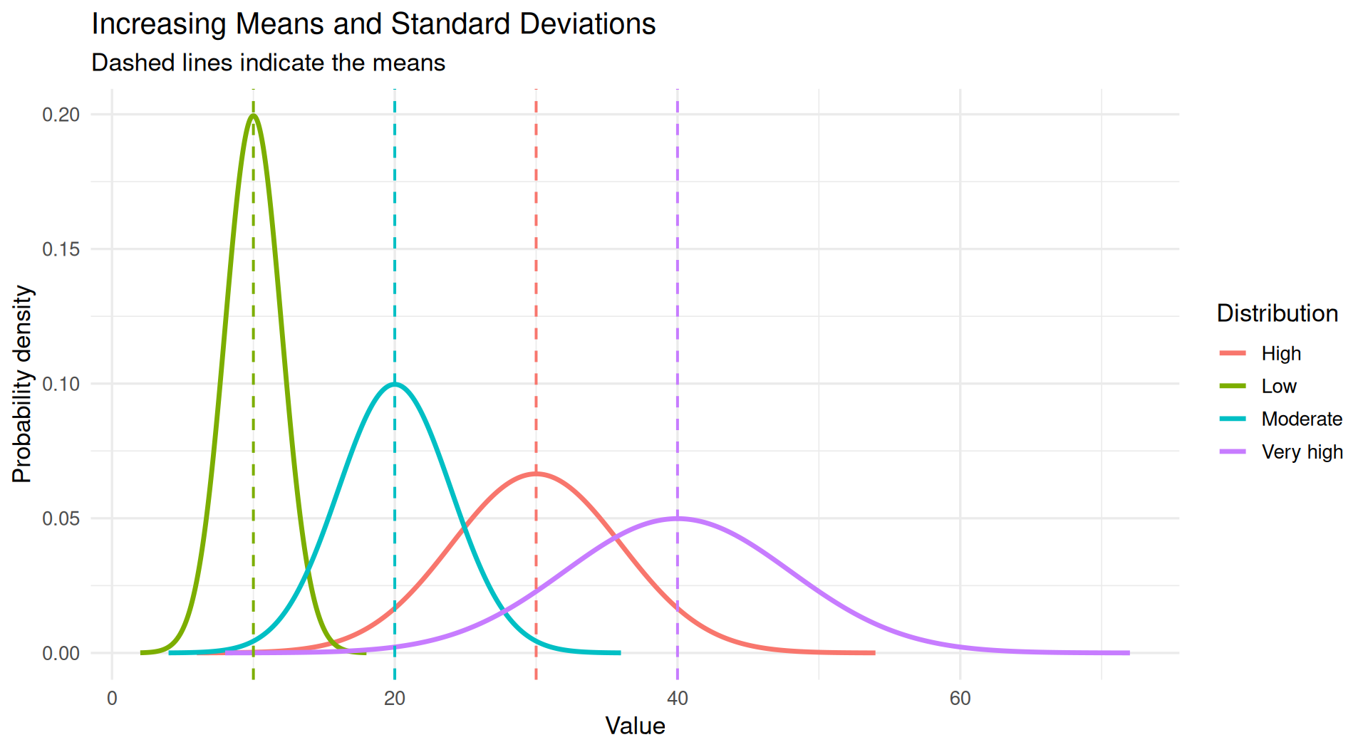
library(ggplot2)
# Define the distributions
params <- data.frame(
group = c("Low", "Moderate", "High", "Very high"),
mean = c(10, 20, 30, 40),
sd = c(2, 4, 6, 8)
)
# Generate density values for each distribution
set.seed(123)
data <- do.call(rbind, lapply(1:nrow(params), function(i) {
x <- seq(
params$mean[i] - 4 * params$sd[i],
params$mean[i] + 4 * params$sd[i],
length.out = 500
)
data.frame(
x = x,
density = dnorm(
x,
mean = params$mean[i],
sd = params$sd[i]
),
group = params$group[i]
)
}))
# Plot the distributions
ggplot(data, aes(x = x, y = density, color = group)) +
geom_line(linewidth = 1.2) +
geom_vline(
data = params,
aes(xintercept = mean, color = group),
linetype = "dashed",
linewidth = 0.7,
show.legend = FALSE
) +
labs(
title = "Increasing Means and Standard Deviations",
subtitle = "Dashed lines indicate the means",
x = "Value",
y = "Probability density",
color = "Distribution"
) +
theme_minimal(base_size = 13)Important
In court
In statistics
“Fail to Reject” Is Not “Accept”
Absence of evidence is not evidence of absence. A tiny study can fail to detect an enormous effect.
Tip
| Term | Meaning |
|---|---|
| \(H_0\) (null) | The boring claim: no difference, no effect, no relationship |
| \(H_1\) (alternative) | What you suspect is happening |
| Test statistic | A number summarizing how far your data is from H₀ |
| p-value | P(data this extreme or more | H₀ is true) |
| α (alpha) | Your threshold, chosen before looking (usually 0.05) |
| Type I error | Rejecting a true H₀ — a false alarm (rate = α) |
| Type II error | Failing to reject a false H₀ — a miss (rate = β) |
| Power | 1 − β: your chance of detecting a real effect |
Four Very Common Errors
❌ “p = 0.03 means there is a 3% chance H₀ is true”
❌ “p = 0.03 means a 97% chance the effect is real”
❌ “p = 0.06 means there is no effect”
❌ “p = 0.001 means the effect is large and important”
What It Actually Says
“If there were truly no effect, data at least this extreme would appear 3% of the time.” That is all. It says nothing about the size or importance of the effect. 📏
Tip
Tip
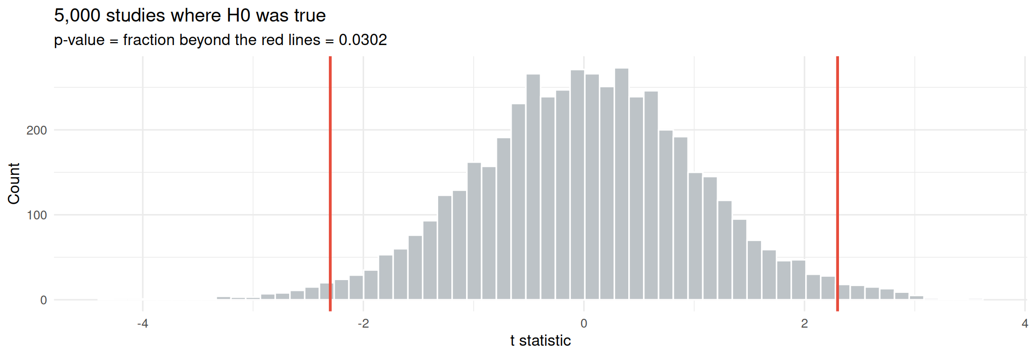
Let’s say we’re testing whether a new drink increases alertness. We have 30 participants, and we measure their alertness before and after drinking the new drink.
We collect the data and find a p-value of 0.03, which is less than our significance level of 0.05. So we reject H₀ and conclude that the new drink increases alertness.
library(tidyverse)
set.seed(301)
# Simulate H0 being TRUE: two groups from the same population
null_ts <- replicate(5000, {
a <- rnorm(20, 100, 15)
b <- rnorm(20, 100, 15) # identical population!
t.test(a, b)$statistic
})
observed <- 2.3 # pretend this is our real study's t statistic
ggplot(tibble(t = null_ts), aes(t)) +
geom_histogram(bins = 60, fill = "#BDC3C7", color = "white") +
geom_vline(xintercept = c(-observed, observed), color = "#E74C3C", linewidth = 1) +
labs(title = "5,000 studies where H0 was true",
subtitle = paste0("p-value = fraction beyond the red lines = ",
round(mean(abs(null_ts) >= observed), 4)),
x = "t statistic", y = "Count") +
theme_minimal(base_size = 12)[1] 0.2450048
[1] 142.2466
Underpowered Studies Are Doubly Dangerous
They usually miss real effects — and when they do hit significance, the estimated effect is exaggerated, because only large flukes clear the bar. 📈
[1] 0.2734048
[1] 0.1367024
Important
Choose the direction before you see the data. Switching to a one-tailed test after a two-tailed test disappoints you is a textbook form of p-hacking. 🚨
Important
Important
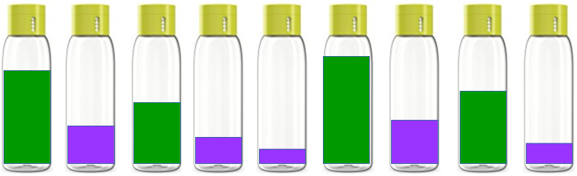
Imagine your company bottles two drinks: green and purple. You suspect that the Green drink bottles are filled to higher levels by the green machine than the Purple machine fills its purple bottles.
Important
Note
We formulate our hypotheses to test the claim that the green and purple drinks are filled to the same levels.
Important
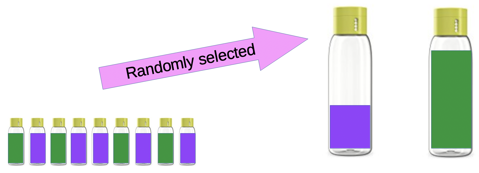
We randomly select 9 bottles of each drink and measure the fill levels. These nine bottles are used to represent the total population of bottles, and to test our hypotheses.
The data is as follows:
t-tests to Compare Means Between Samples
Important
Welch Two Sample t-test
data: green and purple
t = 2.8101, df = 15.404, p-value = 0.01293
alternative hypothesis: true difference in means is not equal to 0
95 percent confidence interval:
1.891901 13.663655
sample estimates:
mean of x mean of y
113.0000 105.2222
Tip
Interpretation of the p-value for Green and Purple Drinks: The p-value = 0.01293 and so we reject the null hypothesis and conclude that there is a statistically significant difference in fill levels between the green and purple drinks.
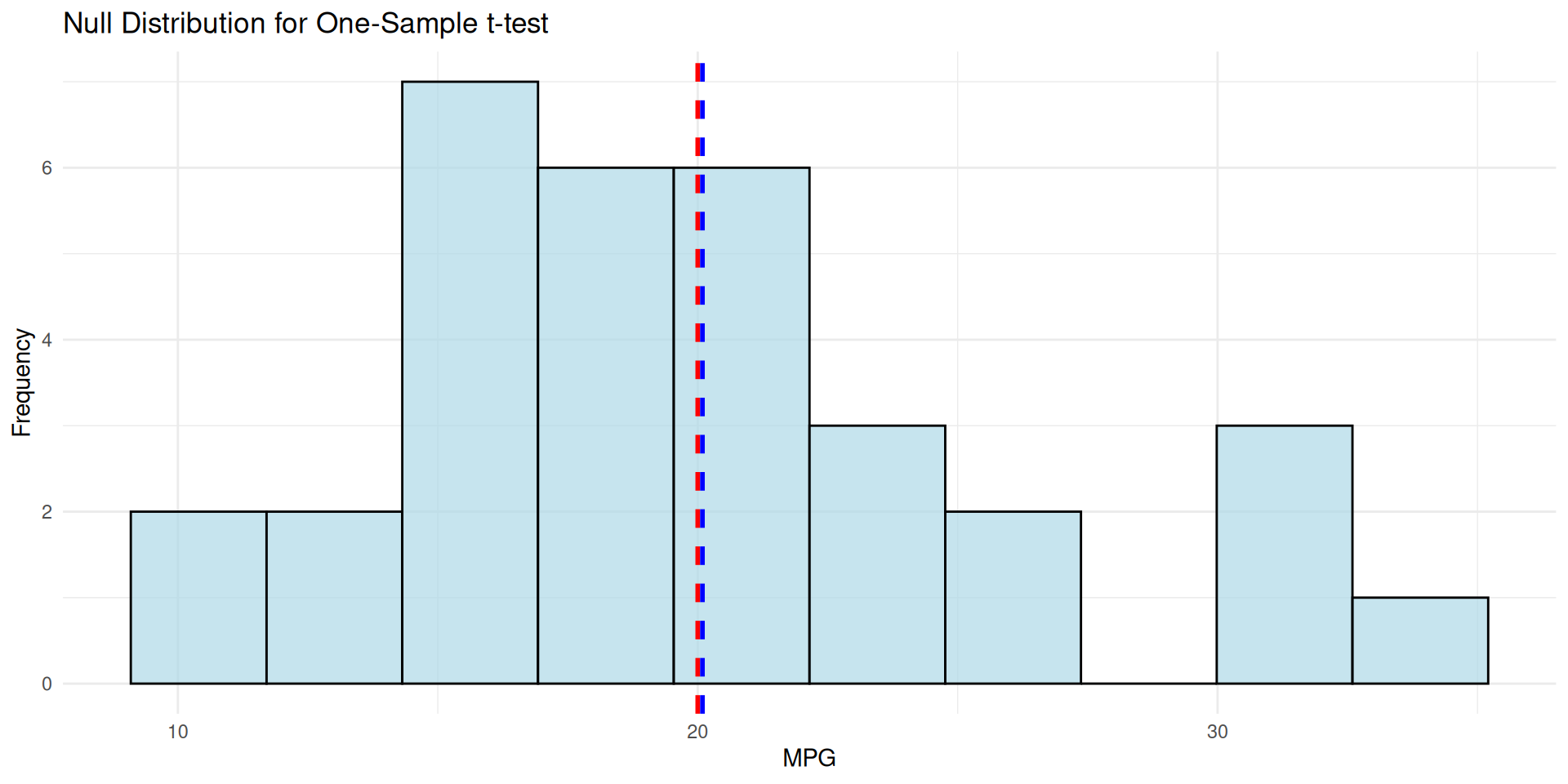
Question: is this sample’s mean different from a specific value?
One Sample t-test
data: mtcars$mpg
t = 0.08506, df = 31, p-value = 0.9328
alternative hypothesis: true mean is not equal to 20
95 percent confidence interval:
17.91768 22.26357
sample estimates:
mean of x
20.09062
library(tidyverse)
# Create a histogram of the sample data
ggplot(mtcars, aes(x = mpg)) +
geom_histogram(bins = 10, fill = "lightblue", color = "black", alpha = 0.7) +
geom_vline(xintercept = 20, color = "red", linetype = "dashed", size = 1) +
geom_vline(xintercept = mean(mtcars$mpg), color = "blue", linetype = "dashed", size = 1) +
labs(title = "Null Distribution for One-Sample t-test",
x = "MPG",
y = "Frequency") +
theme_minimal()mtcars)
Welch Two Sample t-test
data: mpg by am
t = -3.7671, df = 18.332, p-value = 0.001374
alternative hypothesis: true difference in means between group 0 and group 1 is not equal to 0
95 percent confidence interval:
-11.280194 -3.209684
sample estimates:
mean in group 0 mean in group 1
17.14737 24.39231
R defaults to Welch’s t-test, which does not assume equal variances. That is the safer default — keep it. ✅
library(tidyverse)
ggplot(mtcars,
# Note, factor(am) places transmission type
# on the x-axis as a category.
aes(factor(am), mpg,
fill = factor(am))) +
geom_boxplot(alpha = 0.7) +
# geo_jitter() adds the points to box plots
geom_jitter(width = 0.12, size = 2) +
scale_x_discrete(
labels = c("Automatic", "Manual")) +
scale_fill_manual(
values = c("#3498DB", "#E67E22")) +
labs(x = NULL, y = "MPG") +
theme_minimal(base_size = 12) +
theme(legend.position = "none")Important
A PAIRED t-TEST checks whether the mean difference between two matched or related measurements is equal to zero. Good for “before and after” studies, or when the same subjects are measured under two different conditions.
[1] 0.07939414
The p-value for the paired t-test is: 0.00283289
Note
Pairing removes person-to-person variation, so it is far more sensitive. Same data, p drops from 0.079 to 0.003 — the design matters more than the test. 🎯
Important
Calculated as the difference in means divided by the pooled standard deviation.
Used to interpret the practical significance of a t-test result. It helps us understand whether the observed difference between groups is meaningful in a real-world context.
See more about Cohen’s d here: https://en.wikipedia.org/wiki/Effect_size#Cohen’s_d or https://statisticsbyjim.com/basics/cohens-d/.
Chohen’s d is calculated as:
\(d\) = \(\frac{\bar{x}_1 - \bar{x}_2}{s_p}\)
# Cohen's d: the difference in standard deviation units
cohens_d <- function(x, y) {
nx <- length(x); ny <- length(y)
pooled_sd <- sqrt(((nx - 1) * var(x) + (ny - 1) * var(y)) / (nx + ny - 2))
(mean(x) - mean(y)) / pooled_sd
}
manual <- mtcars$mpg[mtcars$am == 1]
automatic <- mtcars$mpg[mtcars$am == 0]
round(cohens_d(manual, automatic), 2)[1] 1.48
| Cohen’s d | Conventional label |
|---|---|
| 0.2 | small |
| 0.5 | medium |
| 0.8 | large |
Important
Always report an effect size and a confidence interval alongside p. With n = 10,000, a meaningless difference gets p < 0.001. 📊
#| echo: true
#| fig-width: 11
#| fig-height: 3.4
# 1. Normality of each group (matters most for small n)
shapiro.test(mtcars$mpg[mtcars$am == 1])$p.value
# 2. Equal variances (only if you use var.equal = TRUE)
var.test(mpg ~ am, data = mtcars)$p.value
# 3. Independence - a design question, not a test!
library(patchwork)
p1 <- ggplot(mtcars, aes(sample = mpg)) +
stat_qq(color = "#2E86C1") + stat_qq_line(color = "#E74C3C") +
labs(title = "Q-Q plot: points on the line = normal") +
theme_minimal(base_size = 11)
p2 <- ggplot(mtcars, aes(mpg)) +
geom_histogram(bins = 12, fill = "#3498DB", color = "white") +
labs(title = "Histogram") + theme_minimal(base_size = 11)
p1 + p2Warning
Normality tests are themselves underpowered at small n and hypersensitive at large n. Look at the Q-Q plot. 👀