ANOVA Hypothesis Testing

The Role of p-values in Making Statistical Decisions

Whatโ€™s On For Today? ๐Ÿ”ฌ

Tip

Formal Statistical Inference

  • ANOVA - comparing three or more groups
  • Post-hoc Tests - which groups differ?
  • Diagnostics - checking the assumptions
  • p-hacking - how testing goes wrong

A p-value answers one narrow question. Know exactly which one.

A New Test

Important

  • ANOVA (Analysis of Variance) is a statistical method used to compare the means of three or more groups.
  • Allows to determine the existence of significant differences between group means without inflating the Type I error rate (More on Error Types later).

Simple Examples of ANOVA Uses:

  • Independent variable is social media use, and you assign groups to low, medium, and high levels of social media use.
  • Dependent variable is hours of sleep per night.
  • Find out if there is a difference in hours of sleep per night

Avoiding Type-I Errors

Important

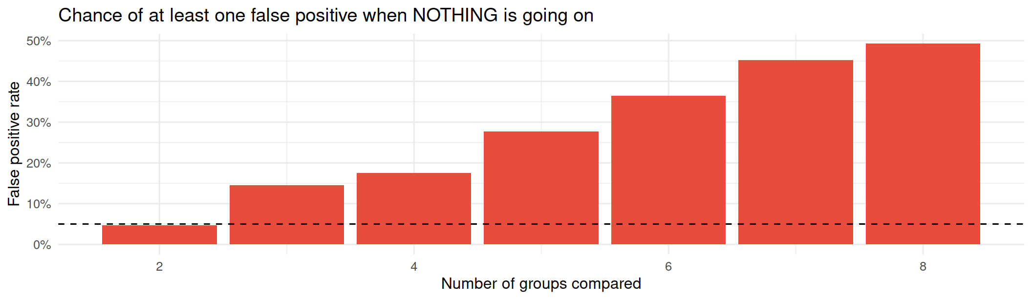
  • When there are more than two groups, running multiple t-tests increases the chance of making a Type I error (false positive).
  • ANOVA avoids this issue by testing all groups simultaneously.

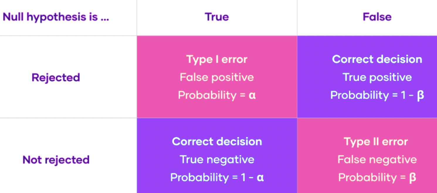
Type Errors:

  • Correct Interpretation of Results
    • Type I Error: Rejecting the null hypothesis when it is true (false positive).
    • Type II Error: Failing to reject the null hypothesis when it is false (false negative).
  • Misinterpretation of Results
    • Type III Error: Correctly rejecting the null hypothesis but for the wrong reason.
    • Type IV Error: Failing to reject the null hypothesis when it is false, and doing so for the wrong reason.

Hey, Is There A, Like, a Huge and Ugly Type-Error Chart??

There Sure Is! Error Types as a Matrix
Assumptions of ANOVA

Tip

  1. Independence of Observations: Each observation should be independent of the others.
  2. Normality: The residuals (errors) should be normally distributed.
  3. Homogeneity of Variance: The variances across groups should be approximately equal.
Why Not Just Run Many t-tests? (code)
library(tidyverse)
set.seed(301)

# Five groups, ALL from the same population - no real differences at all
false_positive <- function(k) {
  groups <- map(1:k, \(i) rnorm(20, 100, 15))
  pairs  <- combn(k, 2)
  ps <- apply(pairs, 2, \(idx) t.test(groups[[idx[1]]], groups[[idx[2]]])$p.value)
  any(ps < 0.05)          # did ANY comparison "find" something?
}

rates <- map_dbl(2:8, \(k) mean(replicate(400, false_positive(k))))

tibble(groups = 2:8, rate = rates) %>%
  ggplot(aes(groups, rate)) +
  geom_col(fill = "#E74C3C") +
  geom_hline(yintercept = 0.05, linetype = "dashed") +
  scale_y_continuous(labels = scales::percent) +
  labs(title = "Chance of at least one false positive when NOTHING is going on",
       x = "Number of groups compared", y = "False positive rate") +
  theme_minimal(base_size = 12)

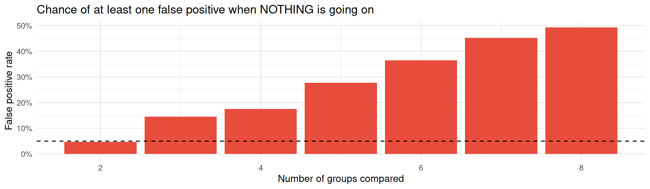
Why Not Just Run Many t-tests (plot)?
Tip

Tip: When you have more than two groups, you should use ANOVA instead of multiple t-tests to avoid inflating the Type I error rate. Type I errors increase with the number of comparisons made. ANOVA controls for this by testing all groups simultaneously.

Letโ€™s Use an Example

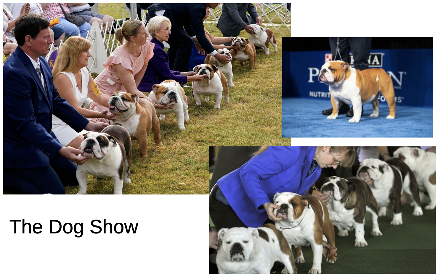
The Dog Show: Description of Problem

Important

  • Imagine that you are hosting a dog show and you want to determine if there are significant differences in the average weights of different dog breeds
  • For this, you will need specific characteristics of the dogs (e.g., breed, weight)
  • You will form groups based on the characteristics of the dogs, and then use ANOVA to compare the average weights across these groups.
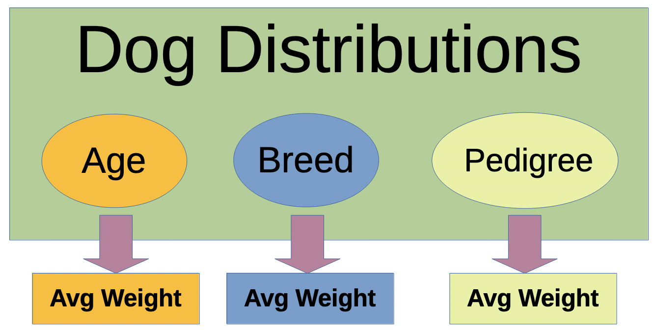
What are the best ways to arrange groups?!

The Dog Show: Letโ€™s Talk About Grouping The Data

For Successful group, we have two main requirements:

  1. Homogeneity of Variance: The variances across groups should be approximately equal.
    • Each group is to be homogeneous or similar by some characteristic.
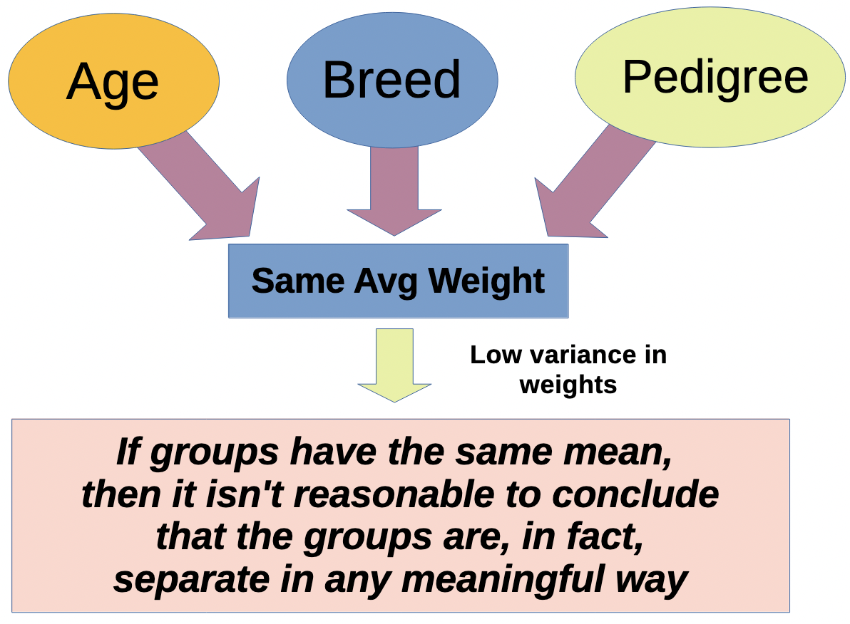
  2. Distinct means: The mean of each group is to be different from the others
    • If groups have the same mean, then they are likely not separate in any meaningful way.
The Dog Show: Bad Group, No Biscuit!

What if the groups are not well-defined?
The Dog Show: Bad Groups
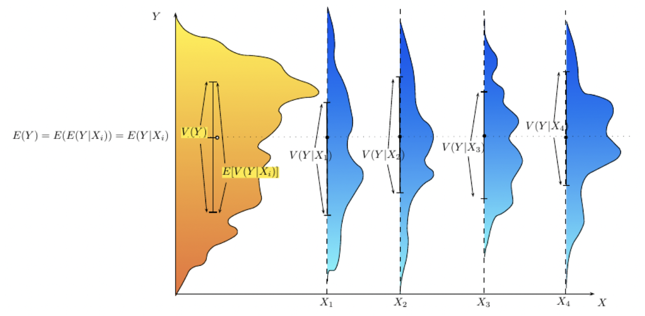
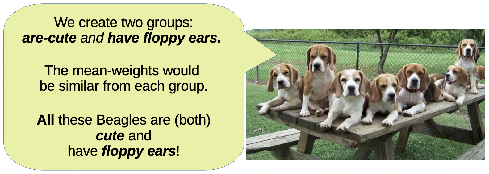
  • Not a fit because all groups are too similar (homogenous). Same mean and same variance.
  • Young vs old, and short-haired vs long-haired
  • This grouping fails to explain the variation in the overall distribution (yellow-orange)

The Dog Show: Better Groups
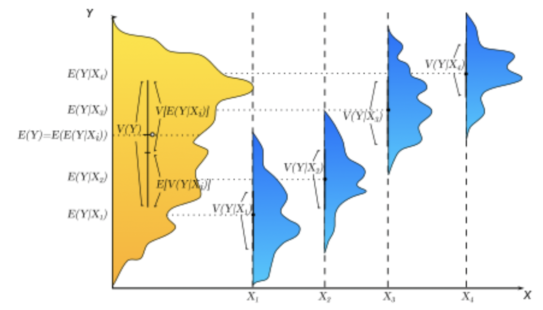
  • A better fit because the groups are distinct and homogeneous. The means are different, and the variances are similar.
  • Pet vs Working breed and less athletic vs more athletic
  • The significant overlap of distributions causes difficulty in distinguishing between the groups.

The Dog Show: Best Grouping
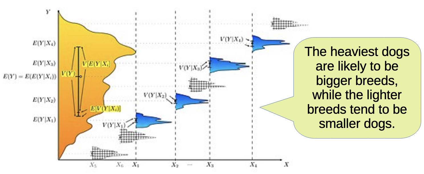
  • A Very good fit because the groups are distinct and homogeneous. The means are different, and the variances are similar.
  • Weight by breed
  • We can discriminate between groups since the distributions are distinct and homogeneous.

Good Groupings
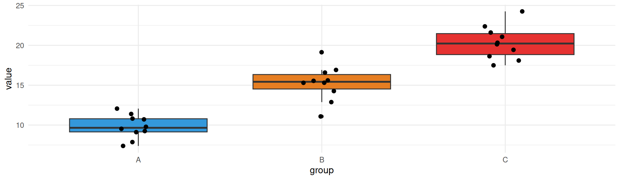
Ideal groupings are distinct and homogeneous

Dogs Groups Selected From a Population
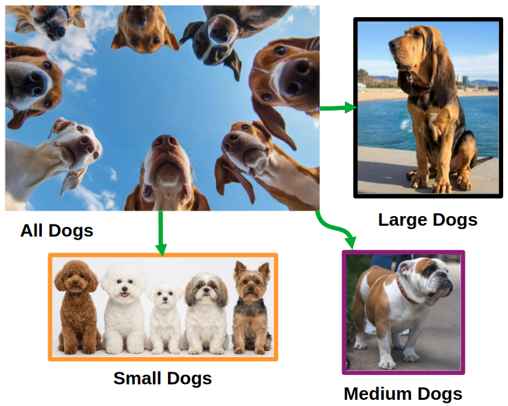
Grouping by dog size: sometimes breeds are not distinct enough to separate the groups. The overlap of distributions causes difficulty in distinguishing the groups.

So What Test?

Important

Want to distinguish between the means of three or more groups.

  • ANOVA is the appropriate test to use in this case.
  • T-tests, works fine for two means, but not more than two means
    • The risks of type error increase with each mean that we are comparing.
    • ANOVA is the appropriate test to use in this case.

One-Way ANOVA: Hypothesis Testing with the Iris data set ๐ŸŒธ

Hypothesis

Hโ‚€: all group means are equal. Hโ‚: * at least one mean differs.

ANOVA asks one question with one test, holding the error rate at alpha.

Tip

Tip: If the p-value is less than the significance level (e.g., 0.05), we reject the null hypothesis and conclude that there is a significant difference between at least two group means.

We cannot tell which mean is different from the others, only that at least one is different. Post-hoc tests are needed to determine which groups differ.

Letโ€™s Hit the Code!

One-Way ANOVA: Run a test

Question: โ€œIs there a statistically significant difference in the mean sepal length among the three species of iris flowers?โ€โ€

model <- aov(Sepal.Length ~ Species, data = iris)
summary(model) 
             Df Sum Sq Mean Sq F value Pr(>F)    
Species       2  63.21  31.606   119.3 <2e-16 ***
Residuals   147  38.96   0.265                   
---
Signif. codes:  0 '***' 0.001 '**' 0.01 '*' 0.05 '.' 0.1 ' ' 1
# The model shows that the p-value is less than alpha = 0.01, 
# indicating that there is a statistically significant difference
# in the mean sepal length among the three species of iris flowers.

Reading the table: the F statistic compares variation between groups to variation within groups. Big F signifies that the groups are far apart from each other relative to their own noise. ๐Ÿ“

A Difference in Means Discovered. Now Where Is It?

Important

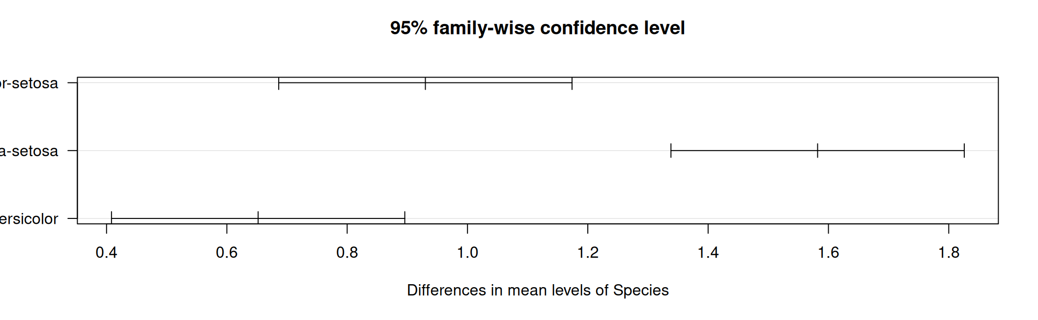
The TukeyHSD(model) function performs Tukeyโ€™s Honestly Significant Difference (HSD) post-hoc test to determine which specific pairs of species differ after conducting an ANOVA.

  • Test: Compare the mean sepal lengths of each pair of species: setosa vs. versicolor, setosa vs. virginica, and versicolor vs. virginica.
    • ANOVA tells us whether there is a significant difference among the species
    • Tukeyโ€™s HSD tells us exactly which species differ from one another

The output provides the estimated difference in means, confidence intervals, and adjusted p-values for each pair.

In simplest terms: The ANOVA tells you whether (IF) any species differ in average sepal length, while Tukeyโ€™s HSD test tells you which (WHAT ONES) specific species differ from one another.

Post-hoc: WHICH Groups Differ? ๐Ÿ”

Question: โ€œWhich specific pairs of iris species have significantly different mean sepal lengths?โ€

tukey <- TukeyHSD(model)
tukey
  Tukey multiple comparisons of means
    95% family-wise confidence level

Fit: aov(formula = Sepal.Length ~ Species, data = iris)

$Species
                      diff       lwr       upr p adj
versicolor-setosa    0.930 0.6862273 1.1737727     0
virginica-setosa     1.582 1.3382273 1.8257727     0
virginica-versicolor 0.652 0.4082273 0.8957727     0

Reading the Tukey Table

Important

Interpreting the Tukey Table: - The diff column shows the difference in means between each pair of groups. - The lwr and upr columns show the lower and upper bounds of the 95% confidence interval for each difference. - The p adj column shows the adjusted p-value for multiple comparisons.

How to interpret each comparison For example, consider versicolor-setosa.

  • diff = 0.930: Versicolor has an average sepal length about 0.93 units greater than setosa.
  • lwr = 0.686 and upr = 1.174: The estimated difference is between 0.686 and 1.174 units at the 95% confidence level.
  • p adj < 0.05: The difference is statistically significant.
  • A useful rule is that if the confidence interval does not include zero, the difference is statistically significant at the corresponding confidence level.

Pos_hoc: WHICH Groups Differ? (plot)

Want to ask: โ€œWhich pairs of iris species have statistically significant differences in their mean sepal lengths?โ€

plot(tukey, las = 1)

Important

Tukeyโ€™s HSD adjusts for all the pairwise comparisons, so these p-values are already corrected. Any interval that misses zero is a real difference. โœ…

Two-Way ANOVA & Interaction ๐Ÿ”€

data(ToothGrowth)
ToothGrowth$dose <- factor(ToothGrowth$dose)

# The * includes both main effects
# AND their interaction
m2 <- aov(len ~ supp * dose,
          data = ToothGrowth)
summary(m2)
            Df Sum Sq Mean Sq F value   Pr(>F)    
supp         1  205.4   205.4  15.572 0.000231 ***
dose         2 2426.4  1213.2  92.000  < 2e-16 ***
supp:dose    2  108.3    54.2   4.107 0.021860 *  
Residuals   54  712.1    13.2                     
---
Signif. codes:  0 '***' 0.001 '**' 0.01 '*' 0.05 '.' 0.1 ' ' 1
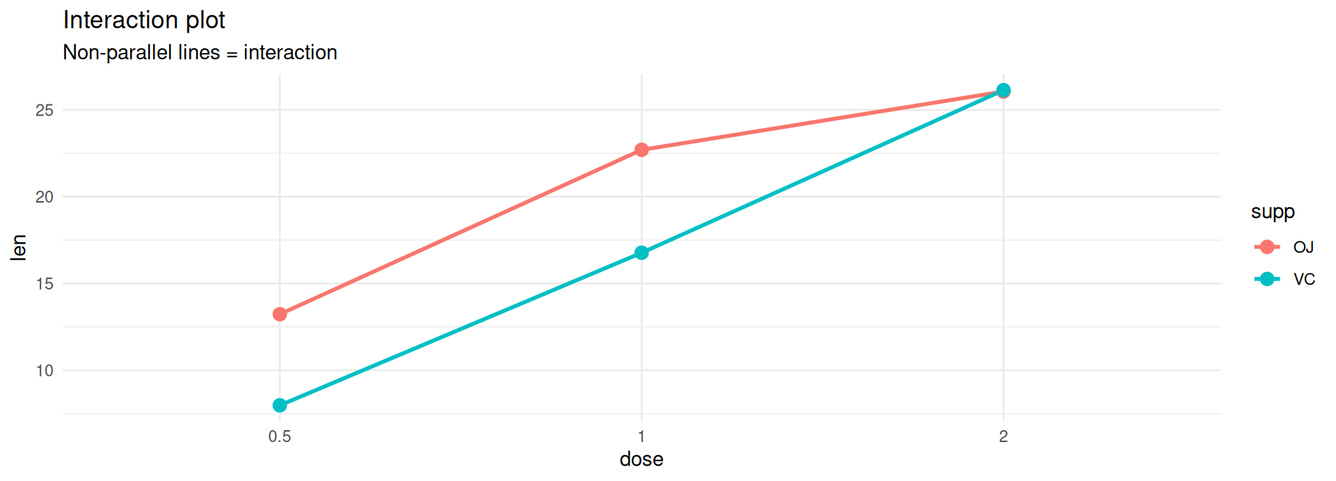
ggplot(ToothGrowth,
       aes(dose, len,
           color = supp,
           group = supp)) +
  stat_summary(fun = mean,
               geom = "line",
               linewidth = 1) +
  stat_summary(fun = mean,
               geom = "point",
               size = 3) +
  labs(title = "Interaction plot",
       subtitle = "Non-parallel lines = interaction") +
  theme_minimal(base_size = 11)

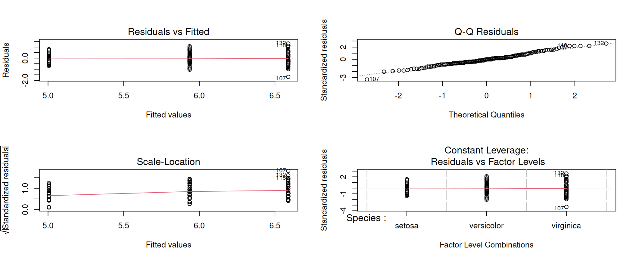
ANOVA Diagnostics ๐Ÿฉบ

par(mfrow = c(2, 2))
plot(model)
par(mfrow = c(1, 1))

Residuals vs Fitted โ€” should be a shapeless cloud (equal variance)

Q-Q Residuals โ€” points should hug the line (normality)

Scale-Location โ€” flat red line means constant spread

Residuals vs Leverage โ€” points past Cookโ€™s distance are influential

MANOVA: Several Outcomes at Once ๐ŸŽญ

# Do species differ across ALL FOUR flower measurements simultaneously?
m_manova <- manova(cbind(Sepal.Length, Sepal.Width,
                         Petal.Length, Petal.Width) ~ Species,
                   data = iris)
summary(m_manova)
           Df Pillai approx F num Df den Df    Pr(>F)    
Species     2 1.1919   53.466      8    290 < 2.2e-16 ***
Residuals 147                                            
---
Signif. codes:  0 '***' 0.001 '**' 0.01 '*' 0.05 '.' 0.1 ' ' 1
# Then look at each outcome separately
summary.aov(m_manova)[[3]]   # third outcome: Petal.Length
             Df Sum Sq Mean Sq F value    Pr(>F)    
Species       2 437.10 218.551  1180.2 < 2.2e-16 ***
Residuals   147  27.22   0.185                      
---
Signif. codes:  0 '***' 0.001 '**' 0.01 '*' 0.05 '.' 0.1 ' ' 1

Tip

Use MANOVA when your outcomes are correlated and you want one overall test before drilling down โ€” it controls the error rate across outcomes. ๐ŸŽฏ

Interactive: ANOVA Builder ๐ŸŽฎ

๐Ÿ“Š ANOVA Builder

Choose a design and click "Generate Code"!

And Now Onto the Ethics of Testing Responsibly

What is P-Hacking?

p-hacking: Ways to Manufacture Significance

๐Ÿšซ Testing many outcomes, reporting the one that worked
๐Ÿšซ Adding participants until p < 0.05, then stopping
๐Ÿšซ Dropping โ€œoutliersโ€ that ruin the result
๐Ÿšซ Trying many subgroups (it works for left-handed users under 30!)
๐Ÿšซ Switching one-tailed after seeing the direction
๐Ÿšซ HARKing โ€” Hypothesizing After Results are Known

Tips for Avoiding P-Hacking

  • Plan your analysis before collecting data
  • Register your study and analysis plan
  • Be transparent about your methods and results
  • Avoid selectively reporting results
  • Use appropriate statistical methods

Letโ€™s See How Easy It Is to P-Hack

set.seed(301)
# Test 20 completely random variables against a random outcome
outcome <- rnorm(50)
# generate 20 random variables and compute 
# their p-values against the outcome
ps <- map_dbl(1:20, \(i) cor.test(rnorm(50), outcome)$p.value)

sum(ps < 0.05)          # "discoveries" from pure noise
[1] 4
round(min(ps), 4)       # the one you would be tempted to publish
[1] 0.0012

Bad Science: Reporting only the tests that worked, but they may have been flukes. The other 19 tests were all noise.

Correcting for Multiple Tests ๐Ÿ›ก๏ธ

# Twenty p-values from twenty tests
raw_p <- c(0.001, 0.008, 0.012, 0.03, 0.04, 0.045,
           0.09, 0.11, 0.20, 0.31, 0.44, 0.52,
           0.60, 0.66, 0.71, 0.78, 0.83, 0.88, 0.92, 0.99)

sum(raw_p < 0.05)                                     # num of uncorrected "discoveries"
[1] 6

Tip

When testing 20 hypotheses, there is an increased chance of obtaining false-positive results. Even if every null hypothesis is true, some tests may produce p-values below 0.05 just by chance. So we can correct for multiple comparisons using methods like Bonferroni, Holm, or Benjamini-Hochberg (BH) to control the family-wise error rate or false discovery rate.

Correcting for Multiple Tests (cont.)

sum(p.adjust(raw_p, method = "bonferroni") < 0.05)    # sum of strictest
[1] 1

Bonferroni Correction: This method adjusts the significance level by dividing it by the number of comparisons. It is the most conservative approach, reducing the chance of false positives but also increasing the chance of false negatives.

Correcting for Multiple Tests (cont.)

sum(p.adjust(raw_p, method = "holm") < 0.05)          # sum of better default
[1] 1

Holm Correction: This method is a step-down version of the Bonferroni correction. It is less conservative and more powerful, while still controlling the family-wise error rate.

sum(p.adjust(raw_p, method = "BH") < 0.05)            # sum of false discovery rate
[1] 1

Benjamini-Hochberg Correction: This method controls the false discovery rate, which is the expected proportion of false positives among all significant tests. It is less conservative than Bonferroni and Holm, making it more powerful for large-scale multiple testing.

Tip

Which to use? holm when every false positive is costly. BH (Benjamini-Hochberg) when you are screening many candidates and can tolerate a known fraction of false leads. ๐ŸŽฏ

Some References for Further Reading (Part 1)

  • P-hacking: A Hidden Threat to Reliable Data Analysis

  • The Brian Wansink Retractions (The Italian Buffet Case Study)

    • The Exposure Analysis: Van der Zee, T., Anaya, J., & Brown, N. J. L. (2017). Statistical heartburn: An attempt to digest four pizza publications from the Cornell Food and Brand Lab. BMC Nutrition, 3(1).
    • Download Open-Access from ResearchGate: Statistical heartburn
    • The Original P-Hacked Paper: Wansink, B., & Payne, C. R. (2014). Eating behavior and obesity at Chinese buffets. Obesity, 22(11), 2307-2312.
      • Note: Because this article was formally retracted by the publisher due to systemic data flaws, an authorized open-access PDF of the final version is not legally hosted by major public archives.
  • Daryl Bemโ€™s Precognition Study & The Failed Replications

    • The Replication Failure: Ritchie, S. J., Wiseman, R., & French, C. C. (2012). Failing the future: Three unsuccessful attempts to replicate Bemโ€™s โ€˜Feeling the Futureโ€™. PLOS ONE, 7(3), e33448.
    • Download Open-Access Publisher PDF via PLOS ONE
    • The Original Paper: Bem, D. J. (2011). Feeling the future: Experimental evidence for anomalous retroactive influences on cognition and affect. Journal of Personality and Social Psychology, 100(3), 407โ€“425. (Note: Published by the APA, this document sits behind a paywall; however, a pre-publication version can frequently be found on academic personal repositories).

Some References for Further Reading (Part 2)

  • The โ€œListening to the Beatlesโ€ Satire
    • The Paper: Simmons, J. P., Nelson, L. D., & Simonsohn, U. (2011). False-positive psychology: Undisclosed flexibility in data collection and analysis allows presenting anything as significant. Psychological Science, 22(11), 1359โ€“1366.
    • Download Open-Access PDF via PubMed

Which Test Do I Need? ๐Ÿ—บ๏ธ

Note

Situation Test R function
One mean vs a value One-sample t t.test(x, mu = )
Two independent means Welch t t.test(y ~ g)
Two paired means Paired t t.test(before, after, paired = TRUE)
3+ means, one factor One-way ANOVA aov(y ~ g)
3+ means, two factors Two-way ANOVA aov(y ~ a * b)
Several outcomes at once MANOVA manova(cbind(...) ~ g)
Which pairs differ Tukey HSD TukeyHSD(model)

Interactive: p-value Simulator ๐ŸŽฎ

๐ŸŽฒ p-value & Power Simulator

Pick a scenario and click "Generate Simulation"!

Knowledge Check ๐Ÿง 

An ANOVA gives p = 0.002 across four groups. What can you conclude?
All four group means differ from each other
At least one group differs โ€” a post-hoc test is needed to say which
The largest and smallest groups differ, and the middle two do not
The differences are large and practically important

Quick Challenges! ๐Ÿง 

Challenge 1: Choosing the Test

You measure blood pressure in 40 patients before and after a 6-week program. Which test?
Two-sample t-test on the 80 measurements
Paired t-test โ€” each patient is their own control
One-way ANOVA with 40 groups
One-sample t-test on the "after" values

Challenge 2: The Significance Trap

Study A (n = 20) reports p = 0.06; Study B (n = 5000) reports p = 0.001. Both estimate the same 0.3-point difference. What is the best reading?
Study B found a real effect; Study A found nothing
Study B's effect is 60 times stronger
Both estimate the same small effect โ€” B just had the precision to resolve it, and 0.3 points may not matter either way
Study A should be rerun until it reaches significance

Challenge 3: Assumptions

Which assumption violation is least fixable by a bigger sample?
Non-normal data
Unequal variances between groups
Non-independent observations (e.g. students clustered in classrooms)
Small expected cell counts

Challenge 4: Write the Code

Write code that tests whether the three PlantGrowth treatment groups differ in weight: check the assumptions, run the ANOVA, and if it is significant, find which pairs differ.

Quick Reference

Task Code
One-sample t t.test(x, mu = 0)
Two-sample (Welch) t.test(y ~ g, data = df)
Paired t t.test(x, y, paired = TRUE)
One-sided alternative = "greater"
One-way ANOVA aov(y ~ g, data = df)
Two-way + interaction aov(y ~ a * b, data = df)
MANOVA manova(cbind(y1, y2) ~ g)
Post-hoc TukeyHSD(model)
Pairwise + correction pairwise.t.test(y, g, p.adjust.method = "holm")
Adjust p-values p.adjust(ps, method = "BH")
Normality shapiro.test(), Q-Q plot
Equal variance var.test(), bartlett.test()
Diagnostics plot(model)
Power / sample size power.t.test(), power.anova.test()