Applications in MANOVA

Multivariate Analysis of Variance

What’s On For Today? 🔬

Tip

Practical Application: Egyptian Skulls

  • Egyptian Skulls dataset
  • R Implementation
  • Visualization techniques
  • Results interpretation

Hands-on Practice

  • Multiple test statistics
  • Post-hoc analysis
  • Real-world examples

What kinds of experiments can we run with manova?

Where Are We Coming From?

t-test

  • Groups: 2
  • Variables: 1 continuous
  • Question: Do two groups differ on one variable?
  • Example: Do males and females differ in height?

ANOVA

  • Groups: 2+
  • Variables: 1 continuous
  • Question: Do multiple groups differ on one variable?
  • Example: Do different treatments affect blood pressure?

MANOVA

  • Groups: 2+
  • Variables: 2+ continuous
  • Question: Do multiple groups differ on multiple variables simultaneously?
  • Example: Do treatments affect both blood pressure AND heart rate ?

The Manova Test: An Overview

Multivariate Analysis of Variance (MANOVA)

  • Extension of ANOVA to multiple dependent variables
  • Tests whether group means differ across multiple continuous variables simultaneously
  • Considers correlations between dependent variables
  • More powerful than running separate ANOVAs when variables are correlated

Key Advantage: Controls for Type I error inflation when testing multiple variables

Important

Real-world Applications

  • Psychology: Do therapy types affect anxiety , depression , and stress simultaneously?
  • Marketing: Do advertisements impact brand awareness , purchase intent , and satisfaction ?

MANOVA Assumptions Overview

Before Running MANOVA: Critical Assumptions to Check!

** Fundamental Requirements**

1 Independence of Observations

2 Multivariate Normality

3 Homogeneity of Covariance

** Additional Considerations**

4 No Extreme Outliers

5 Adequate Sample Size

6 Linear Relationships

Remember: Violating assumptions can lead to invalid conclusions! Always check before interpreting results.

1 Independence of Observations

What it means: Each observation should be independent of all other observations

Good Examples:

  • Different skulls from different individuals (our dataset!)
  • Test scores from different students
  • Patient outcomes from different hospitals
  • Plant growth measurements from different plots

Problematic Examples:

  • Multiple measurements from same individual
  • Family members (genetic correlation)
  • Students within same classroom
  • Repeated measures over time

How to check:

  • Review study design
  • Consider data collection methods
  • Ask: “Could one observation influence another?”

2 Multivariate Normality

What it means: Each group’s data should follow a multivariate normal distribution across all dependent variables

Checking Methods:

  • Shapiro-Wilk test (per variable, per group)
  • Q-Q plots (visual assessment)
  • Mardia’s test (multivariate)
  • Histograms (quick visual check)

When Violated:

  • Skewed distributions
  • Heavy-tailed distributions
  • Bimodal distributions
  • Extreme outliers present

Robustness Note: MANOVA is reasonably robust to normality violations with large samples (n > 30 per group), especially with equal group sizes!

3 Homogeneity of Covariance Matrices

What it means: The covariance matrices should be equal across all groups (Box’s assumption)

Mathematical representation: \[\Sigma_1 = \Sigma_2 = \cdots = \Sigma_k\]

What Equal Covariances Mean:

  • Similar variability (variance is measurement of the spread from the mean) across groups
  • Similar correlations between variables
  • Consistent measurement precision

Testing Methods:

  • Box’s M Test (most common)
  • Visual inspection of covariance matrices
  • Levene’s test (for each variable individually)

3 Homogeneity: Testing & Robustness

What it means: The covariance matrices of the dependent variables are equal across all groups

Box’s M Test Sensitivity:

  • Very sensitive to normality violations
  • Can reject even with minor differences
  • Consider practical significance
  • Often too strict in practice

Robustness Guidelines:

  • Robust with equal group sizes
  • Pillai’s trace most robust when violated
  • Consider Welch’s MANOVA alternatives
  • Violations often acceptable with n ≥ 30

4 No Extreme Outliers

What it means: Extreme values that could distort the analysis should be identified and addressed

Detection Methods:

  • Mahalanobis Distance (multivariate)
  • Box plots (univariate)
  • Scatterplot matrices (visual)

Types: - Univariate, Multivariate, Influential

Handling Options:

  1. Investigate cause
  2. Transform if systematic
  3. Remove if error
  4. Report separately if valid

Rule: Mahalanobis distance > χ²(p, 0.001) = potential outlier

5 Adequate Sample Size

What it means: Sufficient observations per group relative to number of dependent variables

Guidelines:

  • Minimum: n > p per group
  • Better: n ≥ 20 + p per group
  • Best: n ≥ 30 per group

Our Skulls Dataset:

  • 4 variables, 30 per epoch
  • 30 > 24 (20+4) Excellent!

Small Sample Issues:

  • Reduced power & reliability
  • Unreliable covariance estimates
  • Box’s M test problems

Unequal Groups: Keep ratio < 4:1

6 Linear Relationships & Additional Considerations

Linear Relationships:

  • Variables should be linearly related
  • Check with scatterplots
  • Transform if non-linear

Ideal Correlations: r = 0.3 to 0.7

Avoid: - r < 0.3: Use separate ANOVAs - r > 0.9: Multicollinearity issues

Most Robust: Pillai’s Trace Equal groups + n ≥ 30 = Better robustness

When to Use MANOVA

Use MANOVA when:

  • You have 2+ groups (independent variable is categorical)
  • You have 2+ continuous dependent variables
  • Variables are reasonably correlated (but not too highly)
  • You want to control Type I error across multiple tests

Don’t use MANOVA when:

  • Variables are completely uncorrelated (r ≈ 0)
  • Variables are too highly correlated (r > 0.9) - use one variable
  • You have only one dependent variable - use ANOVA
  • Sample size is too small relative to number of variables

MANOVA Hypotheses

Null Hypothesis (H₀): The population mean vectors are equal across all groups

\[H_0: \boldsymbol{\mu}_1 = \boldsymbol{\mu}_2 = \cdots = \boldsymbol{\mu}_k\]

where \(\boldsymbol{\mu}_i = [\mu_{i1}, \mu_{i2}, \ldots, \mu_{ip}]\) is the mean vector for group i

Alternative Hypothesis (H₁): At least one group’s mean vector differs from the others

\[H_1: \text{Not all } \boldsymbol{\mu}_i \text{ are equal}\]

So, Like, What Does That Mean?

  • H₀: All groups have the same average values across all measured variables
  • H₁: At least one group differs from others on at least one variable

Case Study: Egyptian Skulls Dataset

Research Question: Do skull measurements differ across historical epochs?

Dataset Details:

  • 5 Egyptian epochs (time periods)
  • 4 skull measurements per specimen
  • 30 skulls per epoch (150 total)

Variables:

  • mb: Maximum breadth
  • bh: Basibregmatic height
  • bl: Basialveolar length
  • nh: Nasal height

MANOVA Setup:

  • Groups: 5 epochs (c4000BC, c3300BC, c1850BC, c200BC, cAD150)
  • Dependent Variables: mb, bh, bl, nh
  • Research Question: Do skull shapes differ across time periods?
  • **Note: It is always important to know what you are trying to address in your research!

Data Exploration: Loading and Summary

  • data("skulls") loads the measurements; names() verifies available columns.
  • epoch identifies the five time periods; mb, bh, bl, and nh are the four responses.
# Load required libraries
if(!require('tidyverse')) {
  install.packages('tidyverse')
  library('tidyverse')
}

if(!require('HSAUR2')) {
  install.packages('HSAUR2')
  library('HSAUR2')
}

# Load the skulls dataset
data("skulls")
names(skulls)
[1] "epoch" "mb"    "bh"    "bl"    "nh"   

Data Exploration: Summary Statistics

  • Review ranges and quartiles for unexpected values before fitting the model.
  • The summaries are pooled across epochs; compare group-specific patterns in the plots that follow.
# Basic summary
summary(skulls)
     epoch          mb            bh              bl               nh       
 c4000BC:30   Min.   :119   Min.   :120.0   Min.   : 81.00   Min.   :44.00  
 c3300BC:30   1st Qu.:131   1st Qu.:129.0   1st Qu.: 93.00   1st Qu.:49.00  
 c1850BC:30   Median :134   Median :133.0   Median : 96.00   Median :51.00  
 c200BC :30   Mean   :134   Mean   :132.5   Mean   : 96.46   Mean   :50.93  
 cAD150 :30   3rd Qu.:137   3rd Qu.:136.0   3rd Qu.:100.00   3rd Qu.:53.00  
              Max.   :148   Max.   :145.0   Max.   :114.00   Max.   :60.00  

Data Exploration: Means

  • The aggregate() function is used to compute the mean of each measurement for each epoch.
  • The resulting data frame means contains the average values for each measurement across the five epochs.
means <- aggregate(skulls[,c("mb", "bh", "bl", "nh")], 
  list(epoch = skulls$epoch), mean)
means
    epoch       mb       bh       bl       nh
1 c4000BC 131.3667 133.6000 99.16667 50.53333
2 c3300BC 132.3667 132.7000 99.06667 50.23333
3 c1850BC 134.4667 133.8000 96.03333 50.56667
4  c200BC 135.5000 132.3000 94.53333 51.96667
5  cAD150 136.1667 130.3333 93.50000 51.36667

Getting a Visual on the Means?

We note that many of the means seem similar across epochs, but some measurements show more variation than others. This motivates a MANOVA to formally test for differences.

means_long <- means |>
  pivot_longer(
    cols = c(mb, bh, bl, nh),
    names_to = "measurement",
    values_to = "mean"
  )

ggplot(means_long, aes(x = epoch, y = mean, group = 1,  color = epoch)) +
  geom_line() +
  geom_point(size = 3) +
  facet_wrap(~measurement) +
  labs(
    x = "Epoch",
    y = "Mean measurement",
    title = "Mean skull measurements across epochs"  ) +
  theme_minimal()
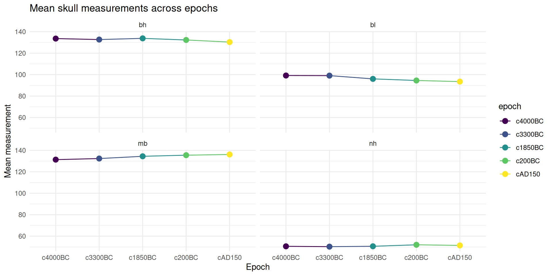
Getting a Visual on the Means Plot
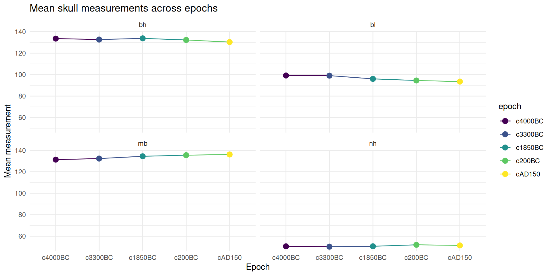
Visualization

Mean Patterns Across Epochs

  • group_by(epoch) and summarise() calculate each measurement’s mean within each epoch.
  • pivot_longer() reshapes the summary for ggplot(), which displays measurements side by side.
  • Compare patterns, but do not infer statistical significance from the plot alone.
# Calculate means by epoch
means_by_epoch <- skulls %>%
  group_by(epoch) %>%
  summarise(across(where(is.numeric), mean, na.rm = TRUE))

# Reshape for plotting
means_long <- means_by_epoch %>%
  pivot_longer(cols = -epoch, names_to = "measurement", values_to = "mean_value")

# Create a vibrant, colorful plot
ggplot(means_long, aes(x = epoch, y = mean_value, fill = measurement)) +
  geom_bar(stat = "identity", position = "dodge", alpha = 0.8) +
  scale_fill_manual(values = c("mb" = "#FF6B6B", "bh" = "#4ECDC4", 
                               "bl" = "#45B7D1", "nh" = "#96CEB4"),
                    labels = c("mb" = "Max Breadth ", "bh" = "Height ", 
                              "bl" = "Length ", "nh" = "Nasal Height ")) +
  labs(title = " Mean Skull Measurements by Epoch",
       subtitle = "Colorful visualization of Egyptian skull evolution over time ",
       x = " Historical Epoch", 
       y = " Mean Value (mm)",
       fill = " Measurements") +
  theme_minimal() +
  theme(
    axis.text.x = element_text(angle = 45, hjust = 1, size = 10),
    plot.title = element_text(size = 16, hjust = 0.5, color = "#2C3E50"),
    plot.subtitle = element_text(size = 12, hjust = 0.5, color = "#7F8C8D"),
    legend.position = "bottom",
    panel.grid.major = element_line(color = "#BDC3C7"),
    panel.background = element_rect(fill = "#FFFFFF")
  )
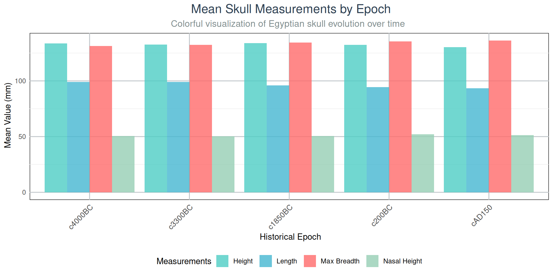
Visualization

Mean Patterns Across Epochs plot
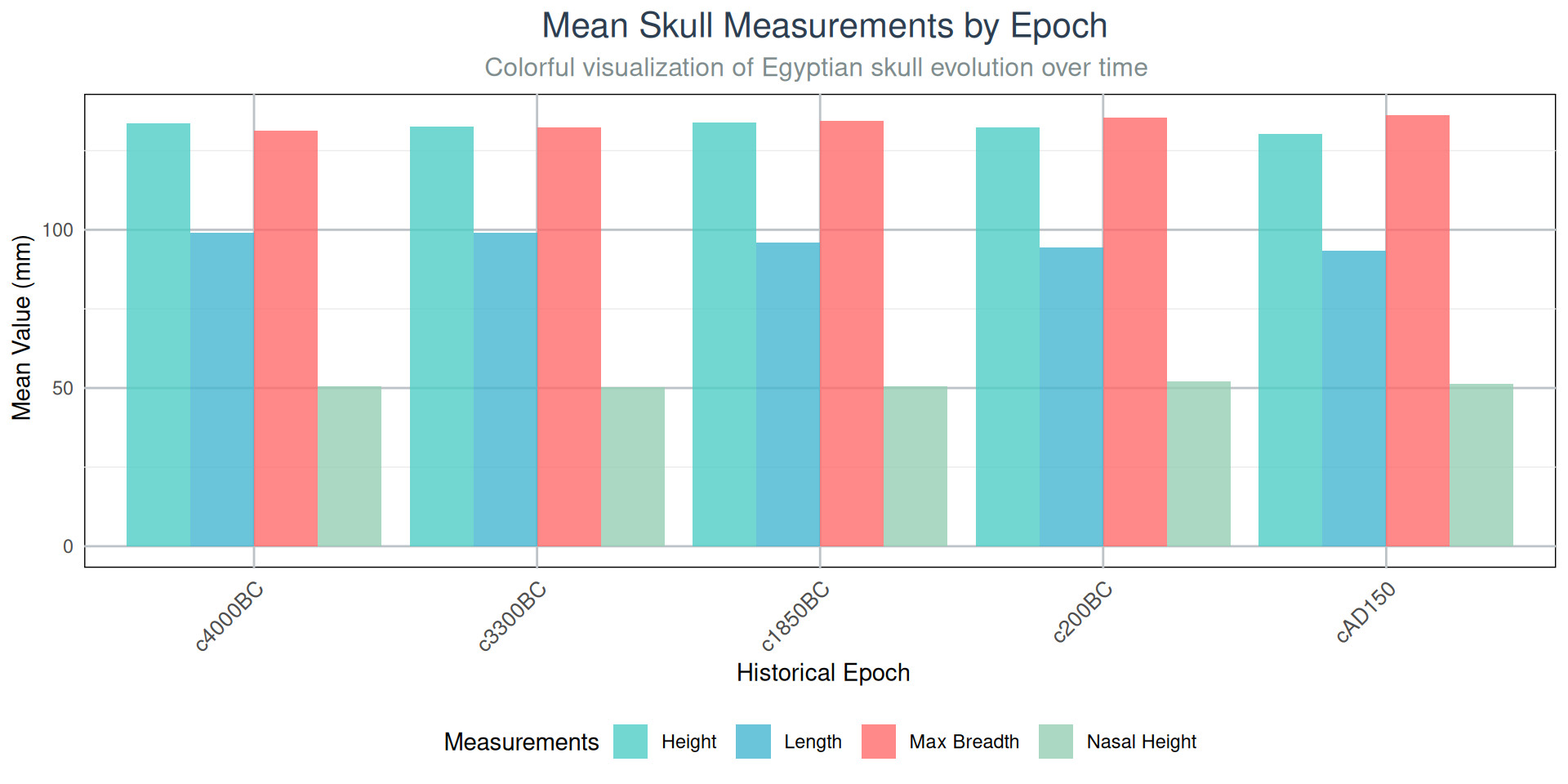
Visual Pattern Analysis

What do you observe?

Important

What the plot suggests

  • Different measurements show different patterns across epochs.
  • Some measurements appear more variable than others.
  • Certain epochs might cluster together.
  • These patterns motivate a MANOVA, but the plot alone does not establish statistical significance.

Key Insight: Visual exploration suggests that skull measurements changed over time , but we need statistical testing to confirm significance!

MANOVA Test Statistics

MANOVA uses multiple test statistics (unlike ANOVA’s single F-statistic):

Wilks’ Lambda (Λ)

  • Most commonly reported
  • Smaller values = greater group differences

Pillai’s Trace

  • Most robust to assumption violations
  • Larger values = greater group differences

Hotelling-Lawley Trace

  • Most powerful when assumptions are met
  • Larger values = greater group differences

Roy’s Greatest Root

  • Most powerful for detecting differences in one dimension
  • Can be liberal (Type I error)

Running MANOVA on the Skulls

Important

Reading the formula

  • The question is whether the five epochs have different mean vectors across the four measurements.
  • cbind() combines the measurements into one multivariate response.
  • epoch is the categorical predictor; convert it to a factor to make that role explicit.
  • manova() fits one joint model, accounting for relationships among the measurements.
skulls$epoch <- factor(skulls$epoch)
skulls.manova <- manova(cbind(mb, bh, bl, nh) ~ epoch, data = skulls)

# Begin with Wilks' Lambda
summary(skulls.manova, test = "Wilks")
           Df   Wilks approx F num Df den Df   Pr(>F)    
epoch       4 0.66359   3.9009     16 434.45 7.01e-07 ***
Residuals 145                                            
---
Signif. codes:  0 '***' 0.001 '**' 0.01 '*' 0.05 '.' 0.1 ' ' 1

Compare MANOVA Test Statistics

Important

  • Wilks’ Lambda is commonly reported; smaller values indicate stronger separation.
  • Pillai’s trace is often preferred when assumptions may be imperfect.
  • These statistics test the overall group effect; they do not identify which epochs differ.
summary(skulls.manova, test = "Pillai")
           Df  Pillai approx F num Df den Df    Pr(>F)    
epoch       4 0.35331    3.512     16    580 4.675e-06 ***
Residuals 145                                             
---
Signif. codes:  0 '***' 0.001 '**' 0.01 '*' 0.05 '.' 0.1 ' ' 1
summary(skulls.manova, test = "Hotelling-Lawley")
           Df Hotelling-Lawley approx F num Df den Df    Pr(>F)    
epoch       4          0.48182    4.231     16    562 8.278e-08 ***
Residuals 145                                                      
---
Signif. codes:  0 '***' 0.001 '**' 0.01 '*' 0.05 '.' 0.1 ' ' 1
summary(skulls.manova, test = "Roy")
           Df    Roy approx F num Df den Df    Pr(>F)    
epoch       4 0.4251    15.41      4    145 1.588e-10 ***
Residuals 145                                            
---
Signif. codes:  0 '***' 0.001 '**' 0.01 '*' 0.05 '.' 0.1 ' ' 1

Interpreting MANOVA Results

Note

The skull measurements differ across epochs: For this dataset, the overall test is significant, so reject the null that all epoch mean vectors are equal.

Important

  • Read the p-value in the selected test-statistic output; a small p-value is evidence against equal mean vectors.
  • This does not mean every epoch differs from every other epoch, or that every measurement changes in the same way.

Important

What the omnibus test does not tell us

  • Which epochs differ?
  • Which variables drive the differences?
  • How large are the differences?

Next steps: Follow-up analyses needed!

Follow-up Analysis: Univariate ANOVAs

Important

  • summary.aov() runs a separate follow-up ANOVA for each response measurement.
  • Use these tests to see which measurements vary by epoch; use planned comparisons to locate group differences.
  • Interpret follow-ups alongside the overall MANOVA, and account for multiple comparisons when testing many pairs.
# Examine each variable separately
summary.aov(skulls.manova)
 Response mb :
             Df  Sum Sq Mean Sq F value    Pr(>F)    
epoch         4  502.83 125.707  5.9546 0.0001826 ***
Residuals   145 3061.07  21.111                      
---
Signif. codes:  0 '***' 0.001 '**' 0.01 '*' 0.05 '.' 0.1 ' ' 1

 Response bh :
             Df Sum Sq Mean Sq F value  Pr(>F)  
epoch         4  229.9  57.477  2.4474 0.04897 *
Residuals   145 3405.3  23.485                  
---
Signif. codes:  0 '***' 0.001 '**' 0.01 '*' 0.05 '.' 0.1 ' ' 1

 Response bl :
             Df Sum Sq Mean Sq F value    Pr(>F)    
epoch         4  803.3 200.823  8.3057 4.636e-06 ***
Residuals   145 3506.0  24.179                      
---
Signif. codes:  0 '***' 0.001 '**' 0.01 '*' 0.05 '.' 0.1 ' ' 1

 Response nh :
             Df Sum Sq Mean Sq F value Pr(>F)
epoch         4   61.2  15.300   1.507 0.2032
Residuals   145 1472.1  10.153               

Interpreting Univariate Results

Important

What we learned

  • mb (Maximum breadth): Significant differences (p < 0.001)
  • bh (Basibregmatic height): Significant differences (p < 0.001)
  • bl (Basialveolar length): Significant differences (p < 0.001)
  • nh (Nasal height): Significant differences (p = 0.003)

All four skull measurements show significant epoch differences!

The results show an association between epoch and skull morphology; this historical comparison alone cannot identify the cause of the differences.

Advanced Visualization

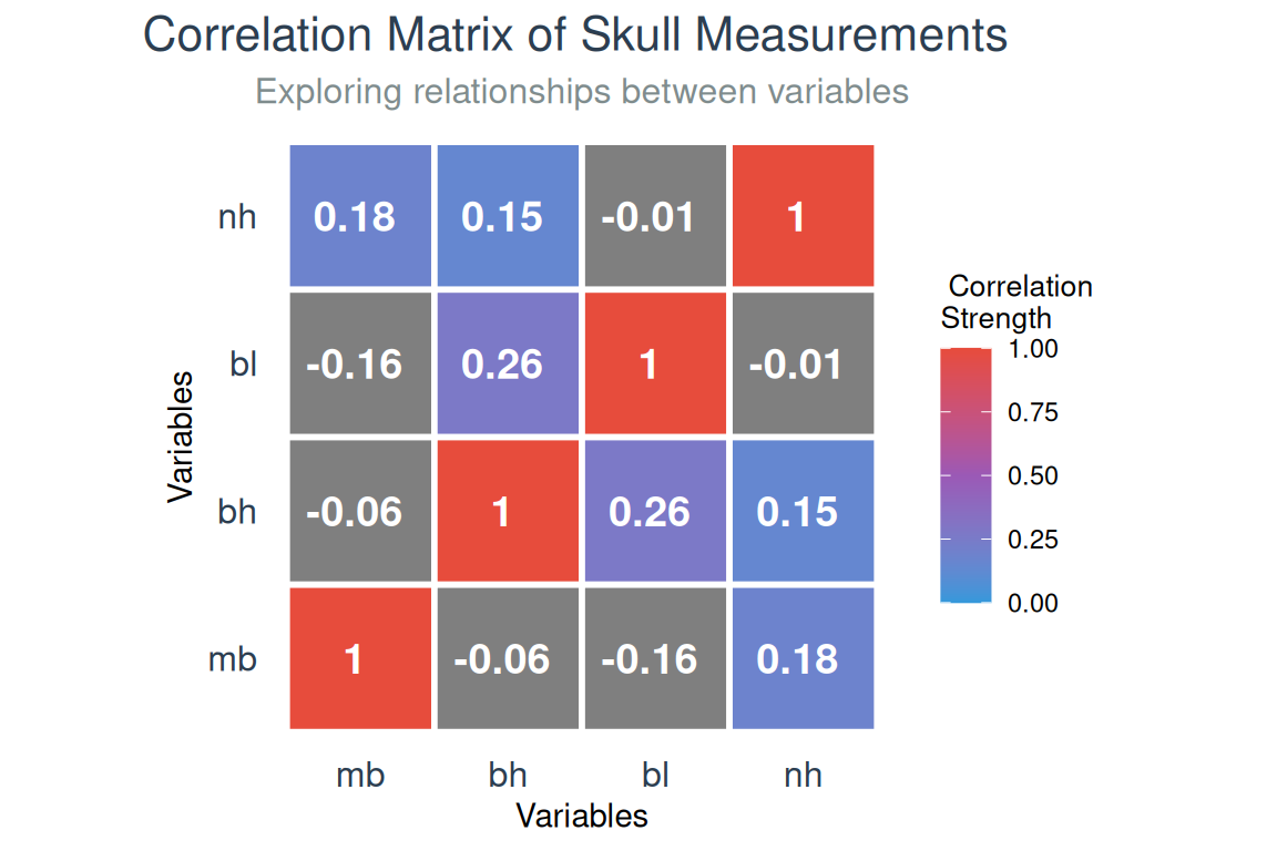
Correlation Heatmap, also known as a Correlation Matrix

# Create correlation matrix for skull measurements
skull_cor <- skulls %>%
  select(mb, bh, bl, nh) %>%
  cor()

# Convert to long format for ggplot
library(reshape2)
skull_cor_long <- melt(skull_cor)

# Create a stunning, colorful heatmap
ggplot(skull_cor_long, aes(Var1, Var2, fill = value)) +
  geom_tile(color = "white", size = 1) +
  geom_text(aes(label = paste0(round(value, 2), 
                               ifelse(value > 0.6, " ", 
                                     ifelse(value > 0.4, " ", " ")))), 
            color = "white", size = 5, fontface = "bold") +
  scale_fill_gradient2(low = "#3498DB", high = "#E74C3C", mid = "#9B59B6", 
                       midpoint = 0.5, limit = c(0,1),
                       name = " Correlation\nStrength") +
  labs(title = "Correlation Matrix of Skull Measurements ",
       subtitle = "Exploring relationships between variables",
       x = "Variables", y = "Variables") +
  theme_minimal() +
  theme(
    plot.title = element_text(size = 16, hjust = 0.5, color = "#2C3E50"),
    plot.subtitle = element_text(size = 12, hjust = 0.5, color = "#7F8C8D"),
    axis.text = element_text(size = 12, color = "#2C3E50"),
    legend.title = element_text(size = 10),
    panel.grid = element_blank(),
    axis.ticks = element_blank()
  ) +
  coord_fixed()
Advanced Visualization

Correlation Heatmap, also known as a Correlation Matrix
Understanding Variable Relationships

Important

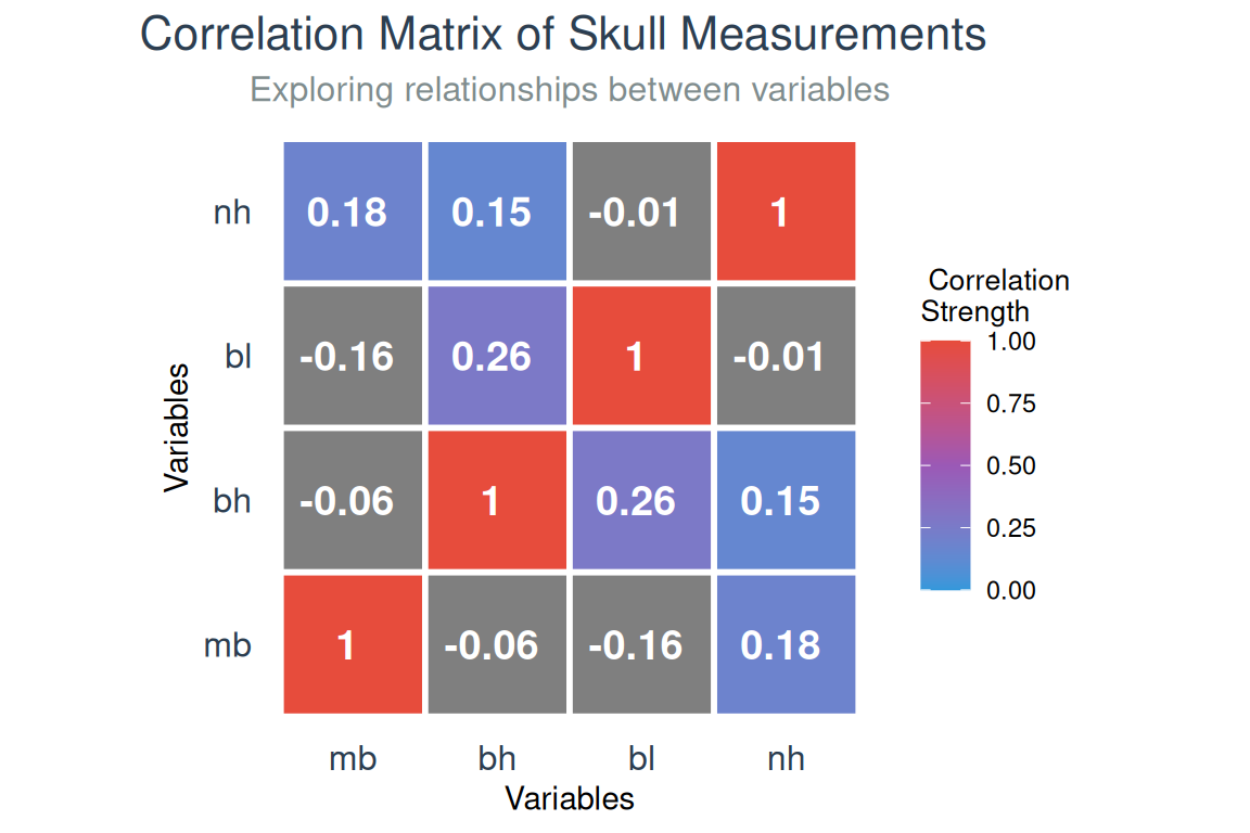
Correlation insights

  • Moderate positive correlations between most measurements
  • Strongest correlation: mb and bl (r = 0.71)
  • Weakest correlation: bh and nh (r = 0.43)

Important

Why this matters for MANOVA

  • Variables are moderately correlated (good for MANOVA)
  • Not too highly correlated (would suggest redundancy)
  • MANOVA accounts for these relationships when testing group differences

Pairwise Epoch Comparison

# Compare just two epochs for demonstration
skulls.manova2 <- manova(cbind(mb, bh, bl, nh) ~ as.factor(epoch), 
                        data = skulls, 
                        subset = as.factor(epoch) %in% c("c4000BC", "c200BC"))

summary(skulls.manova2, test = "Wilks")
                 Df   Wilks approx F num Df den Df    Pr(>F)    
as.factor(epoch)  1 0.69703   5.9766      4     55 0.0004564 ***
Residuals        58                                             
---
Signif. codes:  0 '***' 0.001 '**' 0.01 '*' 0.05 '.' 0.1 ' ' 1

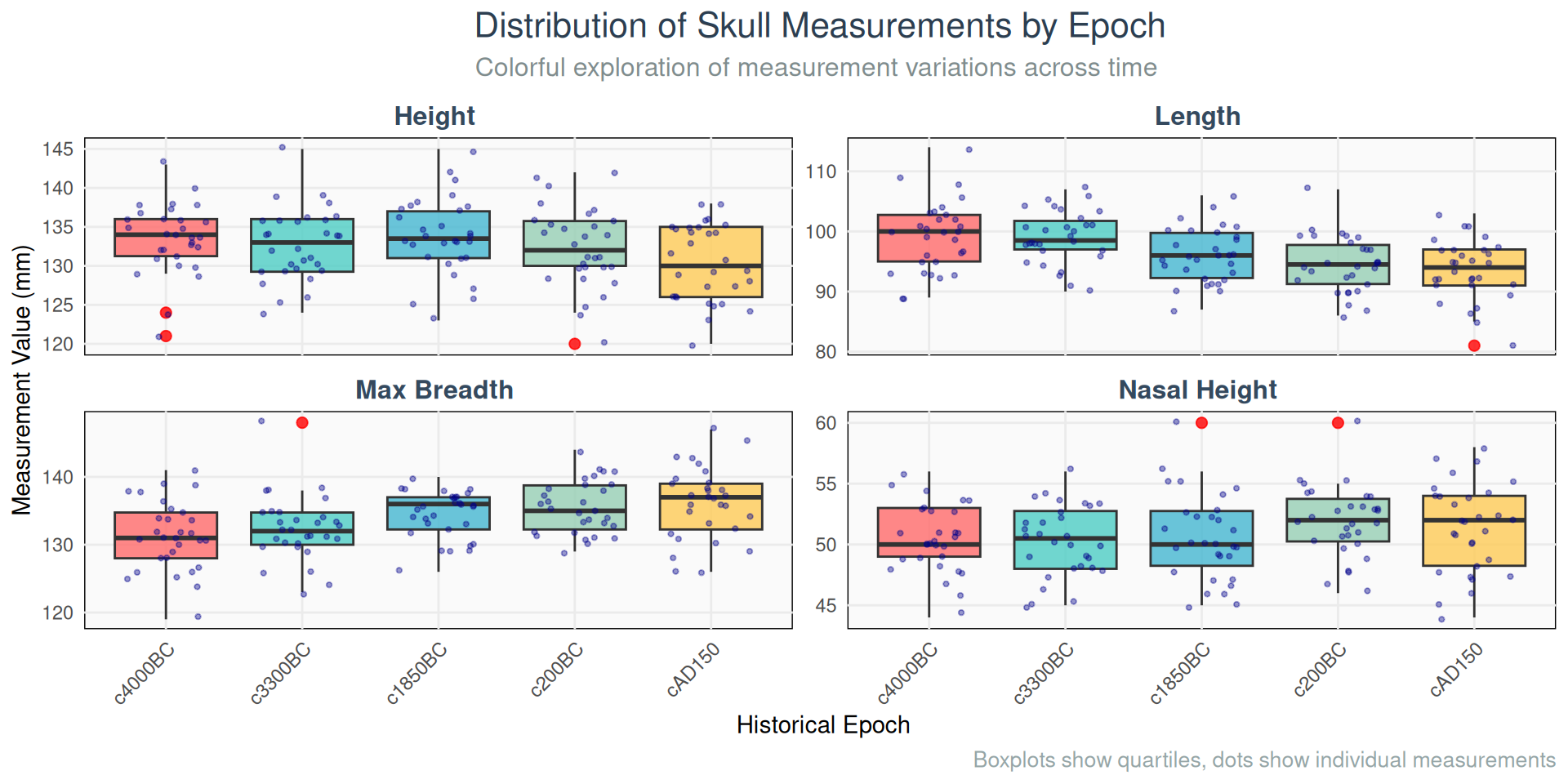
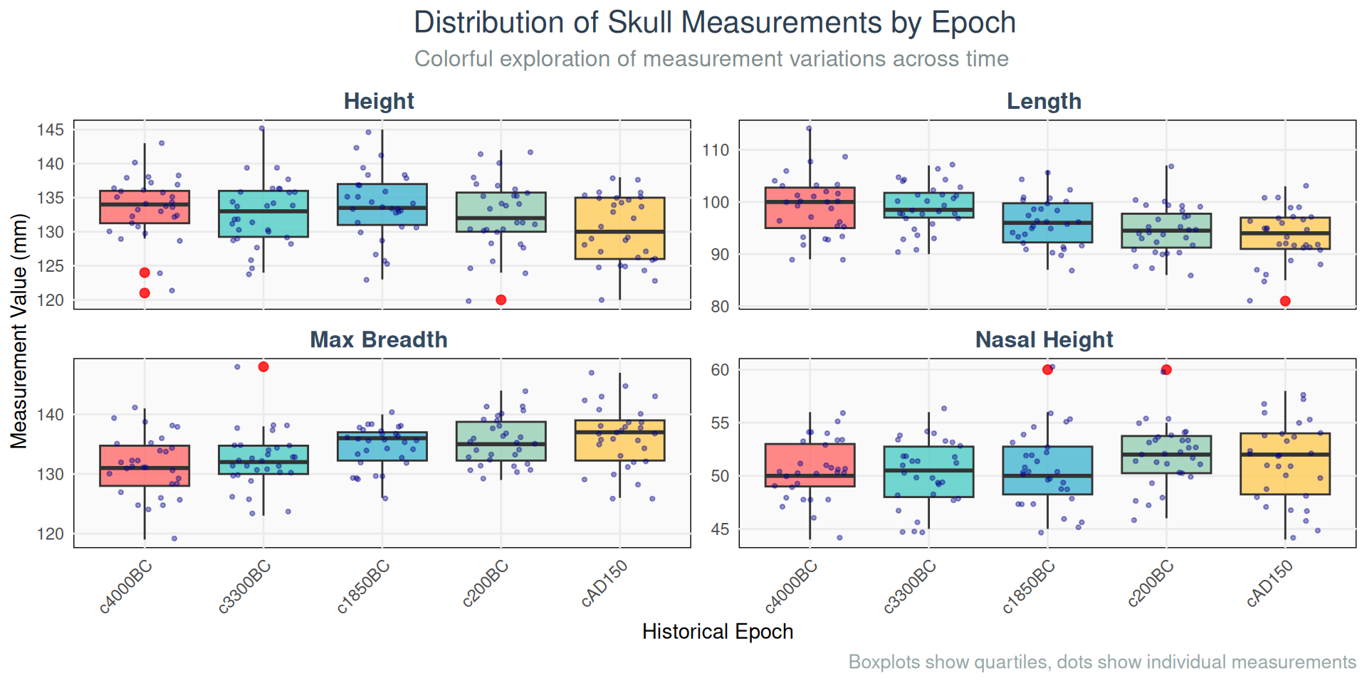
Practical Exercise: Group Means Visualization

# Create vibrant boxplots for each measurement by epoch
skulls_long <- skulls %>%
  pivot_longer(cols = c(mb, bh, bl, nh), 
               names_to = "measurement", 
               values_to = "value") %>%
  mutate(measurement = factor(measurement, 
                             labels = c("bh" = "Height ", "bl" = "Length ",
                                       "mb" = "Max Breadth ", "nh" = "Nasal Height ")))

ggplot(skulls_long, aes(x = epoch, y = value, fill = epoch)) +
  geom_boxplot(alpha = 0.8, outlier.color = "red", outlier.size = 2) +
  geom_jitter(width = 0.3, alpha = 0.4, size = 0.8, color = "darkblue") +
  facet_wrap(~ measurement, scales = "free_y", ncol = 2) +
  scale_fill_manual(values = c("c4000BC" = "#FF6B6B", "c3300BC" = "#4ECDC4", 
                               "c1850BC" = "#45B7D1", "c200BC" = "#96CEB4", 
                               "cAD150" = "#FECA57")) +
  labs(title = " Distribution of Skull Measurements by Epoch ",
       subtitle = "Colorful exploration of measurement variations across time ",
       x = " Historical Epoch", 
       y = " Measurement Value (mm)",
       caption = " Boxplots show quartiles, dots show individual measurements") +
  theme_minimal() +
  theme(
    axis.text.x = element_text(angle = 45, hjust = 1, size = 9),
    plot.title = element_text(size = 16, hjust = 0.5, color = "#2C3E50"),
    plot.subtitle = element_text(size = 12, hjust = 0.5, color = "#7F8C8D"),
    plot.caption = element_text(size = 10, color = "#95A5A6"),
    legend.position = "none",
    strip.text = element_text(size = 12, face = "bold", color = "#34495E"),
    panel.grid.minor = element_blank(),
    panel.background = element_rect(fill = "#FAFAFA")
  )
Practical Exercise: Group Means Visualization Plot
Assumption Check: Egyptian Skulls Dataset

Important

Assumptions to assess

1. Independence of Observations

  • Different skulls from different individuals and time periods
  • No repeated measures or clustering

2. Multivariate Normality

  • Need to test with Shapiro-Wilk or Mardia’s test
  • Visual inspection with Q-Q plots

3. Homogeneity of Covariance Matrices

  • Should test with Box’s M test
  • May be violated but MANOVA is reasonably robust

4. No Extreme Outliers

  • Visual inspection suggests some potential outliers
  • Should check with Mahalanobis distance

5. Adequate Sample Size

  • 30 skulls per epoch and 4 variables provide a good observations-to-responses ratio.

Practical Guidelines

Choosing Test Statistics:

Wilks’ Lambda

  • Default choice
  • Good balance of power and robustness
  • Most commonly reported in literature

Pillai’s Trace

  • Use when assumptions are violated
  • Most robust option
  • Conservative (less Type I error)

Hotelling-Lawley

  • Use when assumptions are clearly met
  • Most powerful option
  • Can be sensitive to violations

Roy’s Greatest Root

  • Use when expecting differences in one primary dimension
  • Can be liberal (more Type I error)

Effect Size in MANOVA

# Calculate eta-squared for overall effect
skulls_aov <- summary.aov(skulls.manova)

# Extract sums of squares for effect size calculation
# This is a simplified approach
cat("Effect sizes (eta-squared) for each variable:\n")
Effect sizes (eta-squared) for each variable:
for(i in 1:4) {
  aov_summary <- skulls_aov[[i]]
  ss_effect <- aov_summary[1, "Sum Sq"]  # Sum of squares for epoch
  ss_total <- sum(aov_summary[, "Sum Sq"])  # Total sum of squares
  eta_sq <- ss_effect / ss_total
  var_name <- c("mb", "bh", "bl", "nh")[i]
  cat(paste(var_name, ": ", round(eta_sq, 3), "\n"))
}
mb :  0.141 
bh :  0.063 
bl :  0.186 
nh :  0.04 

Interpreting Effect Sizes

Eta-squared (η²) Guidelines:

  • Small: η² = 0.01 (1% of variance)
  • Medium: η² = 0.06 (6% of variance)
  • Large: η² = 0.14 (14% of variance)

Our Results Show:

  • All variables have medium to large effects
  • Epoch explains 10-20% of variance
  • Substantial evolutionary changes!

What This Means:

  • Historical periods significantly shaped skull morphology
  • Maximum breadth shows strongest effect
  • Practical significance beyond statistical significance

Remember:

  • Effect size ≠ Statistical significance
  • Both are needed for complete interpretation!

Real-World Applications

Important

Psychology & Education

  • Do teaching methods affect test scores, engagement, and retention simultaneously?
  • Do therapy types impact anxiety, depression, and quality of life measures?

Marketing & Business

  • Do advertisement types influence brand awareness, purchase intent, and customer satisfaction?
  • Do product features affect usability, aesthetics, and functionality ratings?

Biology & Medicine

  • Do species differ across multiple morphological measurements?
  • Do treatments affect multiple health outcomes simultaneously?

Your Turn: Think of a research question in your field that would benefit from MANOVA!

Common Mistakes to Avoid

Important

Running multiple ANOVAs instead of MANOVA

  • Inflates Type I error
  • Ignores variable correlations

Using MANOVA with uncorrelated variables

  • No advantage over separate ANOVAs
  • Wastes statistical power

Ignoring assumptions

  • Can lead to incorrect conclusions
  • Always check assumptions first

Stopping at significant MANOVA

  • Need follow-up analyses to understand which groups/variables differ
  • MANOVA is just the first step!

Practice Time

Important

Try using the following datasets to complete basic manova analyses. Check assumptions, create plots, run the tests, and interpret the results.

  • mtcars dataset: Compare mpg, hp, and wt across different numbers of cylinders (cyl).
  • iris dataset: Compare Sepal.Length, Sepal.Width, Petal.Length, and Petal.Width across species.
  • ToothGrowth dataset: Compare len, supp, and dose across different supplement types and doses.
  • PlantGrowth dataset: Compare weight, group, and treatment across different treatment groups.
  • penguins dataset (from the palmerpenguins package): Compare bill length, bill depth, and flipper length across species and islands.
  • gapminder dataset (from the gapminder package): Compare life expectancy, GDP per capita, and population across continents and years.

Explore MANOVA Further

Use these reproducible examples to compare the skulls analysis with simulated data that has a known group effect.

# Example 1: the four skull measurements across five epochs
data("skulls", package = "HSAUR2")
skulls$epoch <- factor(skulls$epoch)
skull_fit <- manova(cbind(mb, bh, bl, nh) ~ epoch, data = skulls)
summary(skull_fit, test = "Pillai")
summary.aov(skull_fit)

# Example 2: reproducible data with three groups and three outcomes
set.seed(42)
n <- 30
practice <- data.frame(
  group = factor(rep(c("A", "B", "C"), each = n)),
  measure1 = c(rnorm(n, 0, 1), rnorm(n, 0.8, 1), rnorm(n, 1.4, 1)),
  measure2 = c(rnorm(n, 0, 1), rnorm(n, 0.6, 1), rnorm(n, 1.2, 1)),
  measure3 = c(rnorm(n, 0, 1), rnorm(n, 0.2, 1), rnorm(n, 0.4, 1))
)

practice_fit <- manova(cbind(measure1, measure2, measure3) ~ group,
                       data = practice)
summary(practice_fit, test = "Pillai")
summary.aov(practice_fit)
  • Try it: Change n, the group means, or the number of responses. What changes in the MANOVA output?
  • Compare: Set each group’s means to zero to remove the designed shift. A non-significant result is expected on average, but random samples can still produce small p-values.
  • Interpret: Read the multivariate test first, then inspect univariate follow-ups. Simulated data are for learning, not evidence about real populations.

Solution check: With set.seed(42), the simulated example has a significant Pillai test (p approximately 4.13e-08). The follow-up ANOVAs are significant for measure1 and measure2, but not measure3 (p approximately 0.111). In the skulls example, a significant omnibus test means at least one epoch mean vector differs; it does not establish that every pair of epochs differs.

Quick Challenge 1

In manova(cbind(mb, bh, bl, nh) ~ epoch, data = skulls), what does cbind() specify?
Four separate group variables
The four response measurements tested jointly
A request to compare only two epochs
A way to remove correlated measurements

Quick Challenge 2

A significant Pillai test for the skulls model supports which conclusion?
Every epoch differs significantly from every other epoch
At least one epoch mean vector differs across the four measurements
All four measurements changed by the same amount
Epoch caused the observed changes in skull morphology

Quick Challenge 3

What is the purpose of summary.aov(skull_fit) after a significant MANOVA?
It tests whether the covariance matrices are equal
It identifies all significant pairs of epochs automatically
It performs a separate univariate ANOVA for each response
It converts the responses into a single composite score

Quick Challenge 4

What is the primary advantage of using MANOVA over multiple univariate ANOVAs?
It is computationally faster
It provides more detailed post-hoc comparisons
It controls the family-wise error rate across all responses
It requires fewer assumptions

Interactive: Skulls MANOVA Builder

Choose the measurements, test statistic, and epoch scope to generate a runnable R example.

Skulls MANOVA Code Builder

Choose options, then generate the code.

Your Own Research

What Can You Do With MANOVA?

Think about your own research:

  • What datasets might benefit from MANOVA?
  • What variables would you want to test simultaneously?
  • What groups would you compare?

Next Steps:

  • Explore and try Manove on your own data!

Additional Resources

R Packages:

  • HSAUR2: Contains skulls dataset and other examples
  • car: Advanced MANOVA functions and assumption testing
  • MVN: Multivariate normality testing
  • biotools: Box’s M test for homogeneity

Online Resources: