# Replace mydata, x and y with your own data frame and column names

# Clean up workspace
rm(list = ls()) # clear variables from previous work.
graphics.off() # clear out all old plots
cat("\014") # clear the console

library(tidyverse)
mydata <- read_csv("data/groupN_something.csv")   # or paste the tibble from your group's slide
head(mydata)       # what do the first rows look like?
summary(mydata)    # what is the range of each variable?

# Step 1: look before you model
# Note: edit the code to match your variable names and units

plot(mydata$x, mydata$y,
     xlab = "x (units)", ylab = "y (units)",
     main = "y versus x", pch = 19, col = "steelblue")

# Step 2: fit a straight line
model <- lm(y ~ x, data = mydata) # edit x and y to match your variable names
model # the two numbers printed are the intercept and the slope

# Step 3: draw the line on top of the points
abline(model, col = "red", lwd = 2)Discovering Linear Regression
Discovering How Linear Regression Helps in Making Predictions
What’s On For Today? 🔬
Tip
Group Work - discover how linear regression works, and how to use it to make predictions
- The Research Question - What are we trying to determine?
- Evaluating the data - Will this data help us answer the question?
- Plots - What kinds of plots will help us understand the data?
- Prediction - How can we use a plot to make predictions?
- Validation - How can we validate our prediction? Is our prediction even accurate?
- Communication - Communicate our findings to others?
A p-value answers one narrow question. Know exactly which one.
Models: The “Stuff” of Predictive Knowledge
What is a model?
- An (over)-simplified representation of reality, used to make predictions or understand relationships between variables.
- Use variables (predictors) to explain or predict an outcome (response).
- Have shelf lives: they are only valid for the data and context they were built for. Extrapolating beyond that is risky.
- Do not prove causation; they describe associations. Correlation is not causation.

Lots of Different ways to Predict With Models
Linear Models
- Simple linear regression : one variable predicting another
- Multiple linear regression : two or more variables predicting another
- Logistic regression (generalized linear in its parameters) : predicting a binary outcome
Nonlinear Models
- Polynomial regression : curved relationships
- Spline regression : piecewise polynomials for flexible curves
- Generalized additive models (GAMs) : smooth functions of predictors
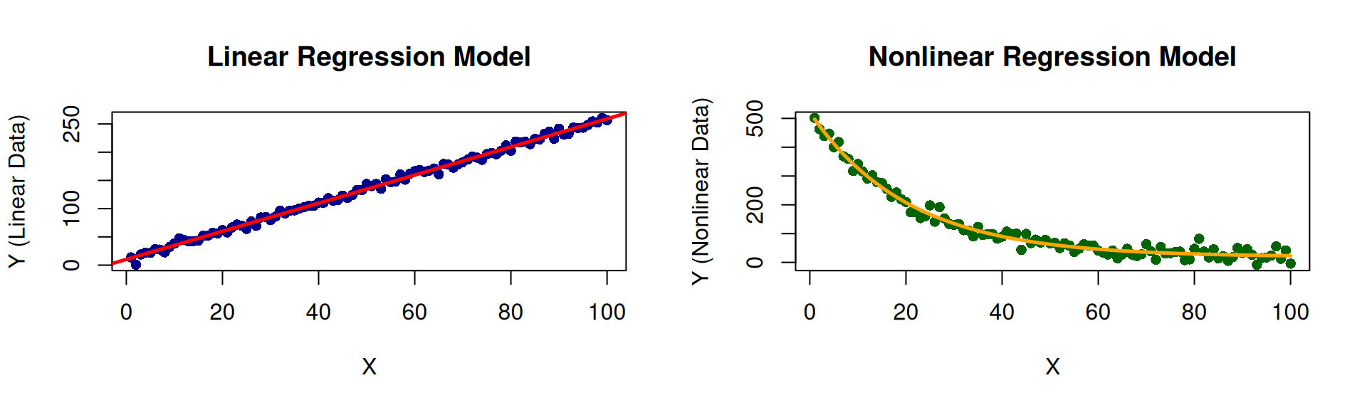
Supervised Models
Note
- Models are trained on labeled data, where the correct answers (labels) are known.
- The goal is to make predictions on new, unseen data.
- Common tasks include classification (predicting categories) and regression (predicting continuous values).
Examples
- Linear Regression (We’re gonna talk about this today!)
- Logistic Regression
- Decision Trees
- Random Forests
- Support Vector Machines (SVM)
- Neural Networks
Unsupervised Models
Note
- Models are trained on unlabeled data, where the correct answers are not known.
- The goal is to discover hidden patterns or structures in the data.
- Common tasks include clustering (grouping similar data points) and dimensionality reduction (reducing the number of variables).
Examples
- K-Means Clustering
- Hierarchical Clustering
- Principal Component Analysis (PCA)
- Independent Component Analysis (ICA)
- Autoencoders
Group Activity
(Oh yeah! This is where the fun begins!)
Activity: Making Predictions from Visualizations
Data → Pattern → Line → Prediction → Model
Today you will discover each step of this chain for yourselves
- Data - What was measured? What are the units? How many observations?
- Pattern - Is there a non-random relationship when we plot one variable against the other?
- Line - Can a straight line summarise that pattern?
- Prediction - Can we use the line to estimate values we did not observe?
- Model - How much should we trust the line? Where does it work, and where does it fail?
We will not define regression. Rather, let the data show you what it does.
How Today Works
Groups of four or five - each group gets its own data and research question
- Read your research question and inspect your data (what are the variables? units? range?)
- Plot your data. Is there a pattern, or does it look random?
- Fit a line with
lm()and draw it on your plot - Predict - use your line to answer the prediction questions for your project
- Test - before reading
summary(), write down what you expect the p-value to say. Were you right? - Discuss your project questions, then the general questions
- Prepare one group member to explain your findings and method to the class (today or next class)
Nothing to submit, just participation.
Groups will present during next class
What Your Group Will Produce
To help you make a prediction and answer your project questions, your group will need to produce the following:
To Address
- A scatterplot of your data with the fitted line drawn on it
- The equation of your line: \(\hat{y} = b_0 + b_1 x\) (with your numbers filled in)
- Your predictions for the values asked about in your project questions
- Your prediction about the p-value written before running
summary(), and what actually happened - Spoken answers to your project questions and the general questions (please be sure to take notes as you work)
Prepare a conversation for the class about your findings
- A fiveminute explanation for the class from your Presenter
- (That’s why you will need the notes!)
Your R Toolkit 🧰
The Six-Step Workflow
Run these in order - and stop after each one to ask “What did I just learn?”
| Step | R command | What you will discover |
|---|---|---|
| 1 | plot(x, y) |
Visual relationship |
| 2 | model <- lm(y ~ x) |
Fitting a mathematical relationship |
| 3 | abline(model) |
Drawing the fitted line |
| 4 | predict(model, newdata) |
Using the line to make predictions |
| 5 | residuals(model) |
Difference between observed and predicted values |
| 6 | summary(model) |
Understanding model results |
The ~ reads as “is modelled by”: lm(y ~ x) means “model y using x”.
Starter Code: Steps 1 to 3
This code will get you started but you might need to add to it in some way (e.g., adding plots, and changing variable names to match your data similar). You may have to look up some of these commands to help you use them. Use ? before the command to get help (e.g., ?plot() for help on making plots, ?lm() for help on the linear model function, or for help on making predictions, use ?predict()).
Starter Code: Steps 4 to 6
# Step 4: use the line to predict y for new x values
new_points <- tibble(x = c(10, 20)) # the column name must match your x variable's name
predict(model, newdata = new_points)
predict(model, newdata = new_points, interval = "prediction")  # a range, not just one number

# Step 5: how far is each point from the line?
residuals(model)
plot(mydata$x, residuals(model), pch = 19,
     xlab = "x", ylab = "Residual (observed - predicted)")
abline(h = 0, lty = 2)                         # a good line leaves residuals scattered around 0

# Step 6: the full report
summary(model)     # find the slope's p-value, and "Multiple R-squared"
Note: Edit this code to match your own variables (e.g., x and y are not x and y in your data)!
Testing Your Prediction with lm()
The experiment
summary(model) tests one specific claim about your line:
- Null hypothesis \(H_0\): the slope is zero (x has no linear relationship with y)
- Alternative \(H_1\): the slope is not zero
Before you run summary() - write down your group’s prediction
- Based on your plot, do you expect the slope to be positive, negative or zero?
- Do you expect the p-value for the slope to be small (below 0.05) or large? Why?
- After running it: were you right? What does the p-value let you conclude, and what does it not tell you?
Code Ideas for Special Situations
# Fit a model WITHOUT one observation
model_all  <- lm(y ~ x, data = mydata)
model_drop <- lm(y ~ x,
                 data = filter(mydata, id != 12))

# Draw both lines on the same plot
plot(mydata$x, mydata$y, pch = 19)
abline(model_all,  col = "red",  lwd = 2)
abline(model_drop, col = "blue", lwd = 2, lty = 2)
legend("topleft", c("All data", "Without #12"),
       col = c("red", "blue"), lty = 1:2)

# Highlight one point
points(mydata$x[12], mydata$y[12],
       col = "orange", pch = 19, cex = 2)
# Predicting far outside your data
predict(model, newdata = tibble(x = 250))
range(mydata$x) # is 250 inside this range?
# A curved model (a parabola) instead of a line
model_curve <- lm(y ~ x + I(x^2), data = mydata)
summary(model_curve)$r.squared
# Draw the curve
grid <- tibble(x = seq(min(mydata$x), max(mydata$x),
length.out = 100))
lines(grid$x, predict(model_curve, grid),
col = "darkgreen", lwd = 2)
# The ggplot way to draw a line
ggplot(mydata, aes(x, y)) + geom_point() +
geom_smooth(method = "lm", se = TRUE)This code could come in useful if your group wants to explore the effect of outliers, extrapolation, or curves.
General Discussion Questions 💬
For Every Group: The Line and the Prediction
Answer these using your data and your model
- Write your fitted equation \(\hat{y} = b_0 + b_1 x\) with your numbers. Say the slope as a sentence that includes the units.
- What does the intercept mean for your data? Is \(x = 0\) a sensible value, or is the intercept only a mathematical anchor for the line?
- What is a residual? Which observation has the largest residual, and can you think of a reason why?
- Is each of your predictions an interpolation (inside the range of your data) or an extrapolation (outside it)? Which do you trust more?
- Why is
interval = "prediction"a wider range than the single predicted value? What does that range say about predicting one individual?
For Every Group: The Model and the p-value
Answer these using your data and your model
- What null hypothesis does the p-value for the slope test? What did your group predict, and what did you find?
- A very small p-value tells you the slope is unlikely to be zero. Does it tell you the line is the right shape? That x causes y? That predictions will be accurate?
- What does R-squared measure? Can a model have a tiny p-value but still make poor predictions?
- What would make you stop trusting your model? (Think: outliers, curves, extrapolation, missing variables.)
- Trace your project through Data → Pattern → Line → Prediction → Model. At which step could things go wrong for your data?
Presenting Your Findings 🎤
Your Group has about 5 minutes. Cover:
- The question - your research question in one sentence (e.g., questions are listed with the data.)
- The data - what was measured, how many observations, the units
- The pattern - show your scatterplot with the fitted line
- The line - your equation, and what the slope means in plain language
- The prediction - one prediction, and how much you trust it
- The test - what you predicted about the p-value, and what
summary()showed - The discovery - the one big lesson your project taught you about regression
- Slides - Use Google slides to show your plots and results. (Who doesn’t like slides!?)
Data → Pattern → Line → Prediction → Model
Come prepared to present your findings to the class next time.
Tip
We will present in the order of the groups, so please be ready to present your findings when your group is called on. Bring slides, code, and notes to class. You will have about 5 minutes to present your findings. Everyone in the group should address one of the questions.
The Projects 🗂️
Which Group Are You?
| Group | Topic | Predictor (x) | Response (y) | n |
|---|---|---|---|---|
| 1 | Study habits | Hours studied | Examination score | 20 |
| 2 | Marketing | Advertising expenditure | Sales revenue | 16 |
| 3 | Real estate | House size | Selling price | 22 |
| 4 | Energy | Outdoor temperature | Electricity consumption | 18 |
| 5 | Human resources | Years of experience | Salary | 16 |
| 6 | Transport | Vehicle speed | Fuel efficiency | 14 |
| 7 | Marketing | Campaign spend | Customer inquiries | 15 |
| 8 | Retail | Daily high temperature | Ice cream sales | 22 |
In addition to added code in the slides, data sets also are available as CSV files Project Downloads Page
Group 1: Study Hours and Examination Scores 📚
Group 1: Research Question and Data
Research question
Is the number of hours a student studies associated with their examination score, and can study hours be used to predict a student’s score?
About the data
Twenty students in one course reported how many hours they studied for the final examination (hours) and their score out of 100 (score). File: data/group1_study_exam.csv, see Project Downloads Page.
Group 1: The Data
| hours | score | hours | score | hours | score |
|---|---|---|---|---|---|
| 2 | 57 | 8 | 54 | 15 | 70 |
| 3 | 37 | 8 | 64 | 16 | 80 |
| 4 | 60 | 10 | 73 | 18 | 80 |
| 5 | 63 | 10 | 82 | 20 | 88 |
| 5 | 59 | 12 | 78 | 22 | 85 |
| 6 | 66 | 12 | 70 | 25 | 95 |
| 7 | 63 | 14 | 71 |
Group 1: Discussion Questions
Your project questions
- Does studying for more hours always guarantee a higher examination score?
- Why might two students who study for the same number of hours receive different examination scores?
- If a student studies for 15 hours, how could the fitted line help predict their examination score?
- Would you trust the prediction equally for a student studying 5 hours and one studying 50 hours? Why?
Hints
- Look for students in the data who studied the same number of hours.
- Try
predict(model, newdata = tibble(hours = c(5, 15, 50))). Does every answer make sense for an exam out of 100?
Group 2: Advertising and Sales 💰
Group 2: Research Question and Data
Research question
Is a company’s monthly advertising expenditure associated with its monthly sales revenue, and can advertising expenditure be used to forecast sales?
About the data
Sixteen months of records for one company: advertising is the monthly advertising budget and sales is that month’s revenue, both in thousands of dollars. File: data/group2_advertising_sales.csv, see Project Downloads Page.
Group 2: The Data
| month | advertising | sales | month | advertising | sales |
|---|---|---|---|---|---|
| 1 | 8 | 167 | 9 | 30 | 287 |
| 2 | 12 | 207 | 10 | 28 | 249 |
| 3 | 15 | 229 | 11 | 35 | 291 |
| 4 | 10 | 191 | 12 | 32 | 308 |
| 5 | 20 | 203 | 13 | 40 | 315 |
| 6 | 22 | 250 | 14 | 38 | 314 |
| 7 | 18 | 197 | 15 | 45 | 337 |
| 8 | 25 | 271 | 16 | 42 | 328 |
Group 2: Discussion Questions
Your project questions
- Does the fitted line suggest that higher advertising expenditure is associated with higher sales?
- If the company increases its advertising budget by $1,000, how could the line help estimate the change in sales?
- Can the company use the line to predict sales for an advertising budget it has never tried?
- Does the fitted line prove that advertising expenditure causes higher sales?
Hints
- Remember the units: an increase of $1,000 is an increase of 1 in
advertising. - Which budgets has the company never tried: $33,000? $100,000? Are those two questions equally safe?
Group 3: House Size and Selling Price 🏠
Group 3: Research Question and Data
Research question
How is the size of a house related to its selling price, and can we estimate the price of a house from its size alone?
About the data
Twenty-two houses sold in one town last year: size (square feet), bedrooms, age (years) and selling price (dollars). Your main analysis uses size and price. File: data/group3_house_prices.csv, see Project Downloads Page.
group3 <- tibble(
  size     = c(1150, 1300, 1420, 1500, 1580, 1650, 1720, 1800, 1880, 1950, 2050,
               2100, 2200, 2280, 2350, 2450, 2600, 2700, 2850, 3000, 3150, 3300),
  bedrooms = c(2, 2, 2, 2, 2, 3, 2, 2, 3, 2, 3, 4, 3, 4, 4, 4, 3, 5, 4, 4, 5, 5),
  age      = c(49, 32, 54, 33, 53, 54, 31, 14, 31, 52, 36, 17, 3, 27, 48, 10, 33, 4, 6, 3, 14, 14),
  price    = c(148000, 191000, 199000, 208000, 171500, 213500, 241500, 246000, 256500, 277000, 250500,
               335500, 343000, 325500, 285000, 361000, 345000, 415000, 439000, 393500, 471000, 433000)
)
Group 3: The Data
| size | bedrooms | age | price | size | bedrooms | age | price |
|---|---|---|---|---|---|---|---|
| 1150 | 2 | 49 | 148000 | 2100 | 4 | 17 | 335500 |
| 1300 | 2 | 32 | 191000 | 2200 | 3 | 3 | 343000 |
| 1420 | 2 | 54 | 199000 | 2280 | 4 | 27 | 325500 |
| 1500 | 2 | 33 | 208000 | 2350 | 4 | 48 | 285000 |
| 1580 | 2 | 53 | 171500 | 2450 | 4 | 10 | 361000 |
| 1650 | 3 | 54 | 213500 | 2600 | 3 | 33 | 345000 |
| 1720 | 2 | 31 | 241500 | 2700 | 5 | 4 | 415000 |
| 1800 | 2 | 14 | 246000 | 2850 | 4 | 6 | 439000 |
| 1880 | 3 | 31 | 256500 | 3000 | 4 | 3 | 393500 |
| 1950 | 2 | 52 | 277000 | 3150 | 5 | 14 | 471000 |
| 2050 | 3 | 36 | 250500 | 3300 | 5 | 14 | 433000 |
Group 3: Discussion Questions
Your project questions
- What does the fitted line suggest about the relationship between house size and selling price?
- Can we estimate the selling price of a house that is 2,500 square feet?
- What does the slope of the line tell us about the relationship?
- Would a house of the same size always sell for the same price? What other variables might matter?
Hints
- The slope is measured in dollars per square foot. Say it as a sentence.
- Compare two houses of similar size with very different prices. What else is different about them?
- Curious? Try
lm(price ~ size + age, data = group3).
Group 4: Temperature and Electricity Use ⚡
Group 4: Research Question and Data
Research question
How does the average daily outdoor temperature relate to household electricity consumption, and can temperature be used to predict how much electricity a household will use?
About the data
Eighteen days between January and May for a household that heats with electricity: average outdoor temperature (°C) and electricity used that day (kWh). File: data/group4_temperature_electricity.csv, see Project Downloads Page.
Group 4: The Data
| temperature | electricity | temperature | electricity | temperature | electricity |
|---|---|---|---|---|---|
| -8 | 54.3 | 1 | 45.4 | 10 | 38.5 |
| -6 | 56.0 | 3 | 45.8 | 12 | 31.4 |
| -5 | 53.2 | 4 | 41.3 | 13 | 36.3 |
| -3 | 49.7 | 6 | 41.5 | 15 | 28.6 |
| -2 | 49.6 | 7 | 37.6 | 16 | 28.7 |
| 0 | 49.0 | 9 | 34.8 | 18 | 21.9 |
Group 4: Discussion Questions
Your project questions
- Why does the fitted line slope downward?
- How does an increase in temperature relate to predicted electricity consumption?
- Can the line help predict electricity consumption at 20°C?
- Would the same relationship necessarily apply during extremely hot weather?
Hints
- What is this household using electricity for on a cold day? On a very hot day?
- What is the warmest day in your data? Is 20°C inside or outside that range? What about 35°C?
Group 5: Experience and Salary 💼
Group 5: Research Question and Data
Research question
How is an employee’s years of experience related to their salary, and how much does the prediction model depend on a single unusual employee?
About the data
Sixteen employees at one company: experience (years) and annual salary (thousands of dollars). Employee 16 is unusual. File: data/group5_experience_salary.csv, see Project Downloads Page.
Group 5: The Data
| employee | experience | salary | employee | experience | salary |
|---|---|---|---|---|---|
| 1 | 1 | 48 | 9 | 7 | 62 |
| 2 | 2 | 48 | 10 | 8 | 62 |
| 3 | 2 | 46 | 11 | 9 | 64 |
| 4 | 3 | 53 | 12 | 10 | 61 |
| 5 | 4 | 53 | 13 | 11 | 65 |
| 6 | 5 | 57 | 14 | 12 | 65 |
| 7 | 5 | 56 | 15 | 13 | 70 |
| 8 | 6 | 55 | 16 | 22 | 165 |
Group 5: Discussion Questions
Your project questions
- Does the fitted line represent all employees equally well?
- What happens to the line when the unusual salary observation is included?
- How does removing the unusual observation change the prediction model?
- Which model would you choose, and what justification would you provide?
Hints
- Fit two models: one with all 16 employees and one with
filter(group5, employee != 16). Draw both lines. - Compare the slopes, and compare the predicted salary for an employee with 10 years of experience.
Group 6: Speed and Fuel Efficiency 🚗
Group 6: Research Question and Data
Research question
How does vehicle speed relate to fuel efficiency, and over what range of speeds can a straight-line model be trusted to predict fuel efficiency?
About the data
One test car driven at a steady speed (km/h) on a test track; efficiency is the fuel efficiency measured at that speed (kilometres per litre, higher is better). File: data/group6_speed_fuel.csv, see Project Downloads Page.
Group 6: The Data
| speed | efficiency | speed | efficiency |
|---|---|---|---|
| 60 | 18.3 | 100 | 15.0 |
| 65 | 17.0 | 105 | 14.7 |
| 70 | 18.2 | 110 | 13.8 |
| 75 | 17.2 | 115 | 14.1 |
| 80 | 16.6 | 120 | 12.9 |
| 85 | 16.4 | 125 | 12.4 |
| 90 | 16.3 | 130 | 11.8 |
Group 6: Discussion Questions
Your project questions
- What does the downward slope tell us about speed and fuel efficiency?
- How can the line estimate fuel efficiency at 95 km/h?
- Does the line suggest that fuel efficiency changes by the same amount for every increase in speed?
- Would you recommend using this model to predict fuel efficiency at 250 km/h?
Hints
- The car was never tested at 95 km/h or at 250 km/h. What is the difference between those two cases?
- Look closely at your residual plot. Do the residuals look random, or do they form a shape?
Group 7: Campaign Spend and Customer Inquiries 📣
Group 7: Research Question and Data
Research question
Is spending more on an advertising campaign associated with more customer inquiries, and how does one unusual campaign affect the prediction model?
About the data
Fifteen online advertising campaigns: spend (hundreds of dollars) and the number of customer inquiries received during the campaign. File: data/group7_campaign_inquiries.csv, see Project Downloads Page.
Group 7: The Data
| campaign | spend | inquiries | campaign | spend | inquiries |
|---|---|---|---|---|---|
| 1 | 5 | 32 | 9 | 25 | 102 |
| 2 | 8 | 45 | 10 | 28 | 108 |
| 3 | 10 | 60 | 11 | 30 | 119 |
| 4 | 12 | 64 | 12 | 32 | 310 |
| 5 | 15 | 75 | 13 | 35 | 132 |
| 6 | 18 | 63 | 14 | 38 | 135 |
| 7 | 20 | 92 | 15 | 40 | 148 |
| 8 | 22 | 87 |
Group 7: Discussion Questions
Your project questions
- What pattern do you notice in the observations?
- How does the unusually high number of inquiries affect the fitted line?
- Which model gives more reasonable predictions: the model with all observations or the model without Campaign 12?
- Should we remove an unusual observation simply because it makes the regression line less representative?
Hints
- Fit two models and compare their slopes, their R-squared values and their p-values.
- Imagine you learn that Campaign 12 was shared by a celebrity. Does that change your answer to question 4? What if it were a typing error?
Group 8: Temperature and Ice Cream Sales 🍦
Group 8: Research Question and Data
Research question
How does the daily high temperature relate to ice cream sales, and is a straight line the right model for predicting sales?
About the data
Twenty-two summer days at a beach-side ice cream shop: daily high temperature (°C) and the number of ice creams sold (sales). File: data/group8_temperature_icecream.csv, see Project Downloads Page.
Group 8: The Data
| temperature | sales | temperature | sales | temperature | sales |
|---|---|---|---|---|---|
| 10 | 64 | 22 | 113 | 30 | 262 |
| 12 | 49 | 23 | 136 | 31 | 261 |
| 13 | 62 | 24 | 127 | 32 | 259 |
| 15 | 82 | 25 | 152 | 33 | 314 |
| 16 | 85 | 26 | 182 | 34 | 318 |
| 18 | 98 | 27 | 182 | 35 | 341 |
| 19 | 93 | 28 | 194 | ||
| 20 | 97 | 29 | 216 |
Group 8: Discussion Questions
Your project questions
- Does the scatterplot suggest that sales increase at a constant rate as temperature increases?
- Does a straight line capture the entire pattern?
- What differences do you notice between the observations and the fitted linear regression line?
- Could a curved line represent the relationship more appropriately?
Hints
- Look at the residuals at the coldest, middle and hottest temperatures. Are they above or below the line?
- Try
lm(sales ~ temperature + I(temperature^2), data = group8)and compare R-squared values.